Performance and Capacity Considerations
Performance and Capacity Considerations
This lesson provides a quick introduction to performance and capacity considerations and discusses why they matter when designing a solution to a machine learning problem.
As we work on a machine learning-based system, our goal is generally to improve our metrics (engagement rate, etc.) while ensuring that we meet the capacity and performance requirements.
Major performance and capacity discussions come in during the following two phases of building a machine learning system:
- Training time: How much training data and capacity is needed to build our predictor?
- Evaluation time: What are the Service level agreement(SLA) that we have to meet while serving the model and capacity needs?
We need to consider the performance and capacity along with optimization for the ML task at hand, i.e., measure the complexity of the ML system at the training and evaluation time and use it in the decision process of building our ML system architecture as well as in the selection of the ML modeling technique.
Complexities consideration for an ML system
Machine learning algorithms have three different types of complexities:
-
Training complexity
The training complexity of a machine learning algorithm is the time taken by it to train the model for a given task.
-
Evaluation complexity
The evaluation complexity of a machine learning algorithm is the time taken by it to evaluate the input at testing time.
-
Sample complexity
The sample complexity of a machine learning algorithm is the total number of training samples required to learn a target function successfully.
Sample complexity changes if the model capacity changes. For example, for a deep neural network, the number of training examples has to be considerably larger than decision trees and linear regression.
The measure of training and evaluation time complexity on a sample data in a ML system
Layered/funnel based modeling approach
To manage both the performance and capacity of a system, one reasonable approach that’s commonly used is to start with a relatively fast model when you have the most number of documents e.g. 100 million documents in case of the query “computer science” for search. In every later stage, we continue to increase the complexity (i.e. more optimized model in prediction) and execution time but now the model needs to run on a reduce number of documents e.g. our first stage could use a linear model and final stage can use a deep neural network. If we apply deep neural network for only top 500 documents, with 1ms evaluation time per document, we would need 500ms on a single machine. With five shards we can do it in around 100ms.
In ML systems like search ranking, recommendation, and ad prediction, the layered/funnel approach to modeling is the right way to solve for scale and relevance while keeping performance high and capacity in check.
The following figure shows an illustration of this multi-layer funnel approach that we will explain in detail in the search ranking system design problem.

Layered model approach for search ranking system
Similarly, the following is an illustration of how an ads relevance system would look in this funnel based approach. We will discuss this in more detail in the ad prediction system chapter.

Funnel approach for an ad prediction system
Training Data Collection Strategies
Learn the training data collection strategies for the machine learning systems you are going to build.
Significance of training data
A machine-learning system consists of three main components. They are the training algorithm (e.g., neural network, decision trees, etc.), training data, and features. The training data is of paramount importance. The model learns directly from the data to create and refine its rules on a given task. Therefore, inadequate, inaccurate, or irrelevant data will render even the most performant algorithms useless. The quality and quantity of training data are a big factor in determining how far you can go in our machine learning optimization task.
A lot of the progress in machine learning - and this is an unpopular opinion in academia - is driven by an increase in both computing power and data. An analogy is to build a space rocket: You need a huge rocket engine, and you need a lot of fuel. - Andrew Ng
Most real-world problems fall under the category of supervised learning problems which require labeled training data. This means that it is necessary to strategically think about the collection of labeled data to feed into your learning system.
Let’s explore strategies that will help in collecting labeled training data for our learning tasks.
Collection techniques
We will begin by looking at the training data collection techniques.
User’s interaction with pre-existing system (online)
In some cases, the user’s interaction with the pre-existing system can generate good quality training data.
We will refer to this technique as online data collection in the course.
For many cases, the early version built for solving relevance or ranking problem is a rule-based system. With the rule-based system in place, you build an ML system for the task (which is then iteratively improved). So when you build the ML system, you can utilize the user’s interaction with the in-place/pre-existing system to generate training data for model training. Let’s get a better idea with an example: building a movie recommender system.
Assume that you are asked to recommend movies to a Netflix user. You will be training a model that will predict which movies are more likely to be enjoyed/viewed by the user. You need to collect positive examples (cases where user liked a particular movie) as well as negative examples (cases where the user didn’t like a particular movie) to feed into your model.
Here, the consumer of the system (the Netflix user) can generate training data through their interactions with the current system that is being used for recommending movies.

Online data collection through a user’s interaction with the system in place
The early version for movie recommendation might be popularity-based, localization-based, rating-based, hand created model or ML-based. The important point here is that we can get training data from the user’s interaction with this system. If a user likes/watches a movie recommendation, it will count as a positive training example, but if a user dislikes/ignores a movie recommendation, it will be seen as a negative training example.
The above discussion was one example, but many machine learning systems utilize the current system in place for the generation of training data.
We will discuss training data generation strategies from the current system in multiple problems in this course, such as search ranking, ads relevance and recommendation systems.
Human labelers (offline)
In other cases, the user of the system would not be able to generate training data. Here, you will utilize labelers to generate good quality training data.
We will refer to this technique as offline data collection in the course.
Let’s take an example of one such case: an image segmentation system for a self-driving car.
Assume that you are asked to perform image segmentation of the surroundings of a self-driving vehicle. The self-driving car will have a camera to take pictures of its surroundings. You will be training a model that will segment these pictures/images into various objects such as the road, pedestrians, building, sidewalk, signal and so on. For this, you will need to provide accurately segmented images of the self-driving car’s surroundings as training data to the model.
Here, the consumer of the system (the person sitting in the self-driving car) can’t generate training data for us. They are not interacting with the system in a way that would give segmentation labels for the images captured by the camera.
In such a scenario, we need to figure out the person/resource that can generate labeled training data for us.
Three such resources are:
-
Crowdsourcing
As the name implies, in crowdsourcing, we outsource a task to a large group of people. Several crowdsourcing websites, such as Amazon Mechanical Turk, where we can get quick results by hiring a lot of people for on-demand tasks, are available for this purpose.
Crowdsourcing can be used to collect training data for relatively simpler tasks. For instance, if you are building an email spam detection system, you would need to label emails as spam or real. This is a simple task that crowd workers can easily do without requiring any special training.

Crowdsourcing the task of generating labeled training data
However, there are cases, like when we have privacy concerns, where we cannot utilize crowdsourcing. If we do not want to show user emails to outsiders, we won’t be using crowdsourcing. Another case where crowdsourcing falls short is when the task at hand requires specialized training. In these cases, we need to have specialized labelers to do the job.
-
Specialized labelers
We can hire specialized/trained labelers who can label data for us according to the given ML task. Let’s say, you have to build a system for the segmentation of driving images for an autonomous vehicle. The trained labelers will use software, such as Label box, to mark the boundaries of different objects in the driving images. One caveat of using specialized labelers is that training them for a specialized task may be time-consuming and costly. The tasks would be delayed until enough labelers have received training.
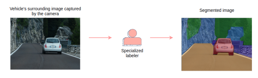
Specialized labellers generating training data
Targeted data gathering
Offline training data collection is expensive. So, you need to identify what kind of training data is more important and then target its collection more. To do this, you should see where the system is failing, i.e., areas where the system is unable to predict accurately. Your focus should be to collect training data for these areas. Continuing with the autonomous vehicle example, you would see where your segmentation system is failing and collect data for those scenarios. For instance, you may find that it performs poorly for night time images and where multiple pedestrians are present. Therefore, you will focus more on gathering and labeling night time images and those with multiple pedestrians. Have a look at the model debugging and testing lesson to find out how to identify areas where the system is performing poorly.
-
Open-source datasets
Generating training data through manual labelers is an expensive and time-consuming way to gather data. So, we need to supplement it with open-source datasets where possible.
For instance, “BDD100K: A Large-scale Diverse Driving Video Database” is an example of an open-source dataset that can be used as training data for this segmentation task. It contains labeled segmented data for driving images.

BDD100K: open source data set for segmentation
We may use more than one of these methods for ways to generating training data. The search ranking chapter is a good example of this.
Additional creative collection techniques
Let’s discuss a few creative ways to collect and expand training data.
-
Build the product in a way that it collects data from user
We can tweak the functionality of our product in a way that it starts generating training data for our model. Let’s consider an example where people go to explore their interests on Pinterest. You want to show a personalized selection of pins to the new users to kickstart their experience. This requires data that would give you a semantic understanding of the user and the pin. This can be done by tweaking the system in the following way:
- Ask users to name the board (collection) to which they save each pin. The name of the board will help to categorize the pins according to their content.
- Ask new users to choose their interests in terms of the board names specified by existing users.
The first step will help you to build content profiles. Whereas, the second step will help you build user profiles. The model can utilize these to show pins that would interest the user, personalizing the experience.

Designing the product in a way that generates training data
-
Creative manual expansion
We can expand training data using creative ways. Assume that we are building a system that detects logos in images (object detection) and we have some images containing the logos we want to detect. We can expand/enhance the training data by manually placing those logos on a different set of images as well. This logo placement can be done in different positions and sizes. The enhanced training data will enable us to build a more robust logo detector model, which will be able to identify logos of all sizes at different positions and from various kinds of images.

Creative manual expansion of training data for logo detection
-
Data expansion using GANs
When working with systems that use visual data, such as object detectors or image segmenters, we can use GANs (generative adversarial networks) to enhance the training data. For instance, consider that we are building an object detector. There are a lot of training images of sunny weather conditions but less of rainy weather. A model trained on this training data may not work well for images with rainy conditions. Here, we can utilize GANs to convert images with sunny weather conditions to rainy weather conditions. This will increase our training data for rainy conditions, resulting in a more robust model.

Training data expansion through GANs: converting images in sunny weather condition to rainy weather condition
Train, test, & validation splits
We have looked at various methods to collect training data. Now it is time to split it into three parts and look at the importance of each split.

The collected training data is split into training data, validation data, and test data
The three parts are as follows:
-
Training data
It helps in training the ML model (fit model parameters).
Model parameters are internal configuration variables of the model. They are learned during model training.
Example of a model parameter: the weights in a neural network.
Model hyperparameters are external configurations of the model that can’t be learned during model training. Their values are selected by using:
- rule of thumb
- trial and error
- heuristics
Example of a model hyperparameter: the learning rate or the number of epochs for training a neural network.
-
Validation data
After training the model, we need to tune its hyperparameters (try different model configurations). This process requires testing the model’s performance on various hyperparameter combinations to select the best one. A simple idea could be to use the training data itself for this task. However, testing the model’s performance on the same data that it was trained on would not give an accurate picture of the model’s generalization ability. A good performance score may be the result of the model overfitting the training data. So we use the validation set while tuning the hyperparameters.
Consider a scenario where you are training a neural network. You want to know the optimal number of epochs. The prediction error on the training set will continue to decrease as you keep on experimenting with a higher number of epochs. However, if you compute the error on the validation set, you would find out that maybe after 300 epochs the prediction error starts to increase, indicating that an epoch number higher than 300 will overfit the training data.

The validation set gives true picture of model’s generalization ability
-
Test data
Now that we have trained and tuned the model, the final step is to test its performance on data that it has not seen before. In other words, we will be testing the model’s generalization ability. The outcome of this test will allow us to make the final choice for model selection. If we had trained several models, we can decide the best ones amongst them and then further see if their performance boost is significant enough to call for an online A/B test.
We pointed out earlier that we need a data set, which the model has not directly learned from, for this test.. As such, training data is out of the question. Validation data is also not a suitable choice. It indirectly impacts the model as it’s used to tune the model hyperparameters. This is where the test data set comes in. Test data is a completely held out data set that provides an unbiased evaluation of the final model, which has been fit on the training dataset.
Points to consider during splitting
- The size of each split will depend on your particular scenario. The training data will generally be the largest portion, especially if you are training a model like a deep neural network that requires a lot of training data. Common ratios used for training, validation and test splits are 60%, 20%, 20% or 70%, 15%, 15% respectively.
- While splitting training data, you need to ensure that you are capturing all kinds of patterns in each split. For example, if you are building a movie recommendation system like Netflix, your training data would consist of users’ interactions with the movies on the platform. After analysing the data, you may conclude that, generally, the user’s interaction patterns differ throughout the week. Different genres and movie lengths are preferred on different days. Hence, you will use the interaction with recommendations throughout a week to capture all patterns in each split.
- Most of the time, we are building models with the intent to forecast the future. Therefore, you need your splits to reflect this intent as well. For instance, in the movie recommendation system example, your data has a time dimension, i.e., you know the users’ interactions with previous movie recommendations, and you want to predict their interactions with future recommendations ahead of time. Hence, you will train the model on data from one time interval and validate/test it on the data from its succeeding time interval, as shown in the diagram below. This will provide a more accurate picture of how our model will perform in a real scenario.

Splitting data for training, validation, and testing
Quantity of training data
As a general guideline, the quantity of the training data required depends on the modeling technique you are using. If you are training a simple linear model, like linear regression, the amount of training data required would be less in comparison to more complex models. If you are training complex models, such as a neural network, the magnitude of data required would be much greater.
Gathering a large amount of training data requires time and effort. Moreover, the model training time and cost also increase as we increase the quantity of training data. To see the optimal amount of training data, you can plot the model’s performance against the number of training data samples, as shown below. After a certain quantity of training data, you can observe that there isn’t any gain in the model’s performance.

Plot of the model’s performance on the validation set against the number of training data samples
Training data filtering
It is essential to filter your training data since the model is going to learn directly from it. Any discrepancies in the data will affect the learning of the model.
-
Cleaning up data
General guidelines are available for data cleaning such as handling missing data, outliers, duplicates and dropping out irrelevant features.
Apart from this, you need to analyze the data with regards to the given task to identify patterns that are not useful. For instance, consider that you are building a search engine’s result ranking system. Cases where the user clicks on a search result are considered positive examples. In comparison, those with just an impression are considered negative examples. You might see that the training data consist of a lot of bot traffic apart from the real user interactions. Bot traffic would just contain impressions and no clicks. This would introduce a lot of wrong negative examples. So we need to exclude them from the training data so that our model doesn’t learn from wrong examples.

Data cleaning: identify and remove unuseful patterns in training data
-
Removing bias
When we are generating training data through online user engagement, it may become biased. Removing this bias is critical. Let’s see why by taking the example of a movie recommender system like Netflix.
The pre-existing recommender is showing recommendations based on popularity. As such, the popular movies always appear first and new movies, although they are good, always appear later on as they have less user engagement. Ideally, the user should go over the whole recommendation list so that he/she can discover the good, new movies as well. This would allow us to classify them as positive training examples so that the model can learn to put them on top, once re-trained. However, due to the user’s time constraints, he/she would only interact with the topmost recommendations resulting in the generation of biased training data. The model hence trained, will continue considering the previous top recommendation to be the top recommendation this time too. Hence, the “rich getting richer” cycle will continue.

Biased training data generated through online user engagement
In order to break this cycle, we need to employ an exploration technique that explores the whole content pool (all movies available on Netflix). Therefore, we show “randomized” recommendations instead of “popular first” for a small portion of traffic for gathering training data. The users’ engagement with the randomized recommendations provides us with unbiased training data. This data really helps in removing the current positional and engagement bias of the system.
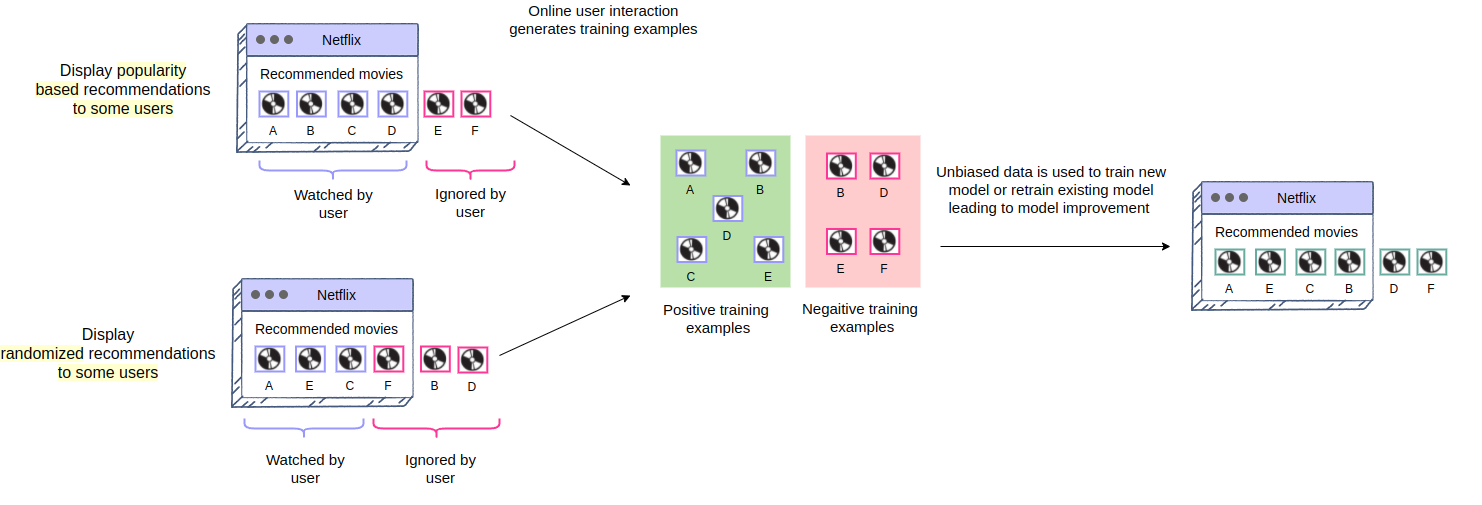
Removing bias through exploration technique
-
Bootstrapping new items
Sometimes we are dealing with systems in which new items are added frequently. The new items may not garner a lot of attention, so we need to boost them to increase their visibility. For example, in the movie recommendation system, new movies face the cold start problem. We can boost new movies by recommending them based on their similarity with the user’s already watched movies, instead of waiting for the new movies to catch the attention of a user by themselves. Similarly, we may be building a system to display ads, and the new ads face the cold start problem. We can boost them by increasing their relevance scores a little, thereby artificially increasing their chance of being viewed by a person.
Online Experimentation
Irrespective of the problem you’re working on, model experimentation and evaluation flow are always critical. In this lesson, we will go over the key steps and concepts in model experimentation and evaluation.
A successful machine learning system should be able to gauge its performance by testing different scenarios. This can lead to more innovations in the model design. For an ML system, “success” can be measured in numerous ways. Let’s take an example of an advertising platform that uses a machine-learning algorithm to display relevant ads to the user. The success of this system can be measured using the users’ engagement rate with the advertisement and the overall revenue generated by the system. Similarly, a search ranking system might take into account correctly ranked search results on SERP as a metric to claim to be a successful search engine. Let’s assume that the first version of the system (v0.1) has been created and deployed.

The initial version of the system is created
Hypothesis and metrics intuition#
At any point in time, the team can have multiple hypotheses that need to be validated via experimentation.
Imagine, for instance, that the team designing an ad prediction system wants to test the hypothesis that increase in the neural network model depth (increase in hidden layers) or width (increase in activation units) will increase latency and capacity but will still have an overall positive effect on user engagement and net ad revenue.
Team desires to test multiple hypotheses to see the impact on the system
Similarly, a team working on designing a search engine wants to test the hypothesis that the pointwise algorithm instead of the pairwise algorithm would positively impact search relevance.

Team desires to test the hypotheses to see the impact on the system
So, to test the hypotheses, should the ML system v0.2 be created and deployed in the production environment? What if the hypothesis intuition is wrong and the mistake becomes costly?
This is where online experimentation comes in handy. It allows us to conduct controlled experiments that provide a valuable way to assess the impact of new features on customer behavior.
Running an online experiment#
A/B testing is very beneficial for gauging the impact of new features or changes in the system on the user experience. It is a method of comparing two versions of a webpage or app against each other simultaneously to determine which one performs better. In an A/B experiment, a webpage or app screen is modified to create a second version of the same page. The original version of the page is known as the control and the modified version of the page is known as the variation.

A/B testing
We can formulate the following two hypotheses for the A/B test:
- The null hypothesis, H0 is when the design change will not have an effect on variation. If we fail to reject the null hypothesis, we should not launch the new feature.
- The alternative hypothesis, H1 is alternate to the null hypothesis whereby the design change will have an effect on the variation. If the null hypothesis is rejected, then we accept the alternative hypothesis and we should launch the new feature. Simply put, the variation will go in production.
Now the task is to *determine if the number of successes in the *variant is significantly better from the control**, i.e., if the conversion caused a positive impact on the system performance. This requires confidently making statements (using statistical analysis) about the difference in the variant sample, even if that difference is small. Before statistically analyzing the results, a power analysis test is conducted to determine how much overall traffic should be given to the system, i.e., the minimum sample size required to see the impact of conversion. Half of the traffic is sent to the control, and the other half is diverted towards the variation.

Traffic split evenly between version A and B
Measuring results#
As visitors are served with either the control or variation/test version of the app, and their engagement with each experience is measured and analyzed through statistical analysis testing. Note that unless the tests are statistically significant, we cannot back up the claims of one version winning over another.
Computing statistical significance#
P-value is used to help determine the statistical significance of the results. In interpreting the p-value of a significance test, a significance level (alpha) must be specified.
📝 The significance level is a boundary for specifying a statistically significant finding when interpreting the p-value. A commonly used value for the significance level is 5% written as 0.05.
The result of a significance test is claimed to be “statistically significant” if the p-value is less than the significance level.
- p <= alpha: reject H0 - launch the new feature
- p > alpha: fail to reject H0 - do not launch the new feature
If an A/B test is run with the outcome of a significance level of 95% (p-value ≤ 0.05), there is a 5% probability that the variation that we see is by chance.

Statistical test analysis shows system B(variation) outperforms system A(control).
Measuring long term effects#
In some cases, we need to be more confident about the result of an A/B experiment when it is overly optimistic.
Back Testing#
Let’s assume that variation improved the overall system performance by 5% when the expected gain was 2%. In the case of the ads prediction system, we can say that the rate of user engagement with the ad increased by 5% in variation (system B). This surprising change puts forth a question. Is the result overly optimistic? To confirm the hypothesis and be more confident about the results, we can perform a backtest. Now we change criteria, system A is the previous system B, and vice versa.

Backtest
We will check all potential scenarios while backtesting:
Do we lose gains? Is the gain caused by an A/B experiment equal to the loss by B/A experiment? Assume that the A/B experiment gave a gain of 5% and B/A experiment gave a loss of 5%. This will ensure that the changes made in the system improved performance.
Long-running A/B tests#
In a few experiments, one key concern could be that the experiment can have a negative long term impact since we do A/B testing for only a short period of time. Will any negative effects start to appear if we do a long term assessment of the system subject to variation?
For example, suppose that for the ad prediction system, the revenue went up by 5% when we started showing more ads to users but this had no effect on user retention. Will users start leaving the platform if we show them significantly more ads over a longer period of time? To answer this question, we might want to have a long-running A/B experiment to understand the impact.
The long-running experiment, which measures long-term behaviors, can also be done via a backtest. We can launch the experiment based on initial positive results while continuing to run a long-running backtest to measure any potential long term effects. If we can notice any significant negative behavior, we can revert the changes from the launched experiment.

Experimental framework stages
Embeddings
Let’s learn what embeddings are and how do we generate them using machine learning techniques.
Embeddings
Embeddings enable the encoding of entities (e.g., words, docs, images, person, ad, etc.) in a low dimensional vector space such that it captures their semantic information. Capturing semantic information helps to identify related entities that occur close to each other in the vector space.
This representation of entities in a lower-dimensional vector space has been of massive help in various ML-based systems. The use of embeddings has seen a major increase because of the recent surge in the use of neural networks and transfer learning.
Usually, they are generated using neural networks. A neural network architectures can be set up easily to learn a dense representation of entities. We will go over a few of such architectures later in this lesson.
Transfer learning refers to transferring information from one ML task to another. Embeddings easily enable us to do that for common entities among different tasks. For example, Twitter can build an embedding for their users based on their organic feed interactions and then use the embeddings for ads serving. Organic interactions are generally much greater in volume compared to ads interactions. This allows Twitter to learn user interests by organic feed interaction, capture it as embedding, and use it to serve more relevant ads.
Another simple example is training word embeddings (like Word2vec) from Wiki data and using them as spam-filtering models.
In this lesson, we will go through some general ways of training neural networks to learn embeddings, using real-world example scenarios of their usage.
Text embeddings
We will go over two popular text term embeddings generation models and examples of their utilization in different ML systems.
Word2vec
Word2vec produces word embeddings by using shallow neural networks (having a single hidden layer) and self-supervised learning from a large corpus of text data. Word2vec is self-supervised as it trains a model by predicting words from other words that appear in the sentence(context). So, it can utilize tons of text data available in books, Wikipedia, blogs, etc. to learn term representation.
Representing words with a dense vector is critical for the majority of Natural language processing (NLP) tasks. Word2vec uses a simple but powerful idea to use neighboring words to predict the current word and in the process, generates word embeddings. Two networks to generate these embeddings are:
- CBOW: Continuous bag of words (CBOW) tries to predict the current word from its surrounding words by optimizing for following loss function:
where nn is the size of our window to look for the corresponding word. It uses the entire contextual information as one observation while training the network. Utilizing the overall context information to predict one term helps generate embeddings with the smaller training dataset. The architecture would look like the following:

Word2vec using CBOW of window size two, i.e., predicting current word using surrounding words
- Skipgram: In this architecture, we try to predict surrounding words from the current word. The loss function will now look like:
where nn is now the size of surrounding words that we are trying to predict using the current word. In training this network, each context pair will result in a different training example that the model tries to predict. This architecture is most helpful when we have a large training set. The model architecture now looks like:

Word2vec using Skip-gram to predict two surrounding words to current word
Example
Any machine learning task that wants to utilize text terms can benefit from this dense embedding vector, which captures word semantic meanings.
Let’s assume that we want to predict whether a user is interested in a particular document given the documents that they have previously read. One simple way of doing this is to represent the user by taking the mean of the Word2vec embeddings of document titles that they haved engaged with. Similarly, we can represent the document by the mean of its title term embeddings. We can simply take the dot product of these two vectors and use that in our ML model.
Another way to accomplish this task is to simply pass the user and the document embedding vector to a neural network to help with the learning task.
Context-based embeddings
Once trained, Word2vec embeddings have a fixed vector for every term. So, a Word2vec embedding doesn’t consider the context in which the word appears to generate its embedding. However, words in a different context can have very different meanings. For example, consider these two sentences:
- I’d like to eat an apple.
- Apple makes great products.
Word2vec will give us the same embedding for the term “apple” although it points to completely different objects in the above two sentences.
So, contextualized information can result in different meanings of the same word, and context-based embeddings look at neighboring terms at embedding generation time. This means that we have to provide contextual information (neighboring terms) to fetch embeddings for a term. In a Word2vec case, we don’t need any context information at the embeddings fetch time as embedding for each term was fixed.
Two popular architectures used to generate word context-based embedding are:
- Embeddings from Language Models (ELMo)
- Bidirectional Encoder Representations from Transformers (BERT)
The idea behind ELMO is to use the bi-directional LSTM model to capture the words that appear before and after the current word.
BERT uses an attention mechanism and is able to see all the words in the context, utilizing only the ones (i.e., pay more attention) which help with the prediction.
We will have an in-depth explanation of these models and architectures in the entity linking chapter. Entity recognition and linking are also a great examples of how contextual embeddings can be very effective; we will discuss this in detail in that chapter.
Visual embedding
Let’s discuss a couple of interesting ways to generate image embedding.
Auto-encoders
Auto-encoders use neural networks consisting of both an encoder and a decoder. They first learn to compress the raw image pixel data to a small dimension via an encoder model and then try to de-compress it via a decoder to re-generate the same input image. The last layer of encoder determines the dimension of the embedding, which should be sufficiently large to capture enough information about the image so that the decoder can decode it.
The combined encoder and decoder tries to minimize the difference between original and generated pixels, using backpropagation to train the network. The network will look like the following:

Auto-encoder model architecture for generating visual embeddings
Once we have trained the model, we only use the encoder (first N network layers) to generate embeddings for images.
Auto-encoders are also an example of self-supervised learning, like Word2vec, as we can use an image data set without any label to train the model and generate image embeddings.
Visual supervised learning tasks#
Visual supervised learning tasks such as image classification or object detection, are generally set up as convolution layers, pooling layers, and fully connected network layers, followed by final classification(softmax) layers. Let’s consider the example of the ImageNet VGG16 model that is shown in the figure below. The input passes through a set of convolution, pooling, and fully connected layers to the last softmax layer for the final classification task. The penultimate layer before softmax captures all image information in a vector such that it can be used to classify the image correctly. So, we can use the penultimate layer value of a pre-trained model as our image embedding.

VGG16 architecture
An example of image embedding usage could be to find images similar to a given image.
Another example is an image search problem where we want to find the best images for given text terms, e.g. query “cat images”. In this case, image embedding along with query term embedding can help refine search relevance models.
Learning embeddings for a particular learning task#
Most of our discussion so far has been about training a general entity embedding that can be used for any learning task. However, we can also embed an entity as part of our learning task. The advantage of this embedding is a specialized one for the given prediction task. One important assumption here is that we have enough training data to be able to learn such representation during model training. Another consideration is that training time for learning the embedding as part of the task will be much higher compared to utilizing a pre-trained embedding.
Let’s consider an example where we are trying to predict whether a user will watch a particular movie based on their historical interactions. Here, utilizing movies that the user has previously watched as well as their prior search terms can be very beneficial to the learning task. We can do this by embedding sparse vector of movies and terms in the network itself, as shown in the image below. We will also discuss this specialized embedding usage in detail in the recommendation system chapter.

Network/Relationship-based embedding
Most of the systems have multiple entities, and these entities interact with each other. For example, Pinterest has users that interact with Pins, YouTube has users that interact with videos, Twitter has users that interact with tweets, and Google search has both queries and users that interact with web results.
We can think of these interactions as relationships in a graph or resulting in interaction pairs. For the above example, these pairs would look like:
- (User, Pin) for Pinterest
- (User, Video) for YouTube
- (User, Tweet) for Twitter
- (Query, Webpage) for Search
- (Searcher, Webpage) for Search
In all the above scenarios, the retrieval and ranking of results for a particular user (or query) are mostly about predicting how close they are. Therefore, having an embedding model that projects these documents in the same embedding space can vastly help in the retrieval and ranking tasks of recommendation, search, feed-based, and many other ML systems.
We can generate embeddings for both the above-discussed pairs of entities in the same space by creating a two-tower neural network model that tries to encode each item using their raw features. The model optimizes the inner product loss such that positive pairs from entity interactions have a higher score and random pairs have a lower score. Let’s say the selected pairs of entities (from a graph or based on interactions) belong to set A. We then select random pairs for negative examples. The loss function will look like
$Loss=max(\sum_{(u,v)\in A}dot(u,v) - \sum_{(u,v)\notin A}dot(u,v))$

Two tower model to optimize inner product loss for user and item embeddings