1 Introduction

Notes

Problem: binary relationship from inputs to outputs
Algorithm: procedure mapping each input to a single output
- An algorithm solves a problem if it returns a correct output for each and every problem input
Correctness:
- For small inputs: can use case analysis
- For arbitrarily large inputs: algorithm either is recursive or loop in some way. Use induction.

Efficiency: how fast does an algorithm produce a correct output?

Count the number of fixed time operations algorithm takes to return
Asymptotic Notation: ignore constant factors and low order terms

input	constant	logarithmic	linear	log-linear	quadratic	polynomial	exponential
$n$	$Θ(1)$	$Θ(log n)$	$Θ(n)$	$Θ(n log n)$	$Θ(n^2)$	$Θ(n^c )$	$2^Θ(n^c)$
$1000$	$1$	$≈ 10$	$1000$	$≈ 10,000$	$1,000,000$	$1000^c$	$2^1000 ≈ 10^301$
Time	$1 ns$	$10 ns$	$1 µs$	$10 µs$	$1 ms$	$10^{(3c-9)} s$	$10^281 millenia$

Model of Computation: what operations on the machine can be performed in $O(1)$ time.
- Machine word: block of w bits (w is word size of a w-bit Word-RAM)
- Memory: Addressable sequence of machine words
- Processor supports many constant time operations on a $O(1)$ number of words (integers):
 - integer arithmetic: (+, -, *, //, %)
 - logical operators: (&&, ||, !, ==, <, >, <=, =>)
 - bitwise arithmetic: (&, |, «, », …)
 - Given word a, can read word at address a, write word to address a
Data Structure: a way to store non-constant data, that supports a set of operations
- A collection of operations is called an interface
- Example:
  - Sequence: Extrinsic order to items (first, last, nth)
  - Set: Intrinsic order to items (queries based on item keys)
- Data structures may implement the same interface with different performance
Example: Static Array - fixed width slots, fixed length, static sequence interface
- StaticArray(n): allocate static array of size n initialized to 0 in $Θ(n)$ time
- StaticArray.get_at(i): return word stored at array index i in $Θ(1)$ time
- StaticArray.set_at(i, x): write word x to array index i in $Θ(1)$ time

2 Data Structures

Notes

Data Structure Interfaces

A data structure is a way to store data, with algorithms that support operations on the data
Collection of supported operations is called an interface (also API or ADT)
Interface is a specification: what operations are supported (the problem!)
Data structure is a representation: how operations are supported (the solution!)

Sequence Interface (L02, L07)

Maintain a sequence of items (order is extrinsic)
Ex: ($x_0$, $x_1$, $x_2$, . . . , $x_{n-1}$) (zero indexing)
use n to denote the number of items stored in the data structure
Supports sequence operations:

Type	Interface	Specification
Container	`build(X)`	given an iterable X, build sequence from items in X
	`len()`	return the number of stored items
Static	`iter_seq()`	return the stored items one-by-one in sequence order
	`get_at(i)`	return the $i^{th}$ item
	`set_at(i, x)`	replace the $i^{th}$ item with x
Dynamic	`insert_at(i, x)`	add $x$ as the $i^{th}$ item
	`delete_at(i, x)`	remove and return the $$i^{th}$ item
	`insert_fist(x)`	add $x$ as the first item
	`delete_first(x)`	remove and return the first item
	`insert_last(x)`	add $x$ as the last item
	`delete_last(x)`	remove and return the last item

Special case interfaces:
- stack: insert_last(x) and delete_last()
- queue: insert_last(x) and delete_first()

Set Interface (L03-L08)

Sequence is about extrinsic order, set is about intrinsic order
Maintain a set of items having unique keys (e.g., item x has key x.key)
Set or multi-set? We restrict to unique keys for now.
Often we let key of an item be the item itself, but may want to store more info than just key

Supports set operations:

Type	Interface	Specification
Container	`build(X)`	given an iterable X, build sequence from items in X
	`len()`	return the number of stored items
Static	`find(k)`	return the stored item with key k
Dynamic	`insert(x)`	add x to set (replace item with key x.key if one already exist)
	`delete(x)`	remove and return the stored item with key k
Order	`iter_ord()`	return the stored items one-by-one in key order
	`find_min()`	return the stored item with smallest key
	`find_max()`	return the stored item with largest key
	`find_next(k)`	return the stored item with smallest key larger than k
	`find_prev(k)`	return the stored item with largest key smaller than k

Special case interfaces:
dictionary: set without the Order operations

Array Sequence

Array is great for static operations! get at(i) and set at(i, x) in Θ(1) time!
But not so great at dynamic operations…
For consistency, we maintain the invariant that array is full.
Then inserting and removing items requires:
- reallocating the array
- shifting all items after the modified item

Sequence Data Structure	API Type			Worst Case $O(\cdot)$
Array	Container	Static	Dynamic
API	`build(x)`	`get_at(i)` `set_at(i)`	`insert_first(x)` `delete_first()`	`insert_last(x)` `delete_last()`	`insert_at(i, x)` `delete_at(i)`
Array	$n$	$1$	$n$	$n$	$n$

Linked List Sequence

Pointer data structure (this is not related to a Python “list”)
Each item stored in a node which contains a pointer to the next node in sequence
Each node has two fields: node.item and node.next
Can manipulate nodes simply by relinking pointers!
Maintain pointers to the first node in sequence (called the head)
Can now insert and delete from the front in $Θ(1)$ time! Yay!
(Inserting/deleting efficiently from back is also possible; you will do this in PS1)
But now get_at(i) and set_at(i, x) each take $O(n)$ time… :(
Can we get the best of both worlds? Yes! (Kind of…)

Sequence Data Structure	API Type			Worst Case $O(\cdot)$
Array	Container	Static	Dynamic
API	`build(x)`	`get_at(i)` `set_at(i)`	`insert_first(x)` `delete_first()`	`insert_last(x)` `delete_last()`	`insert_at(i, x)` `delete_at(i)`
Linked List	$n$	$n$	$1$	$n$ # 1 if we keep track of tail	$n$

Dynamic Array Sequence

Make an array efficient for last dynamic operations
Python “list” is a dynamic array
Idea! Allocate extra space so reallocation does not occur with every dynamic operation
Fill ratio: $0 ≤ r ≤ 1$ the ratio of items to space
Whenever array is full ($r = 1$), allocate $Θ(n)$ extra space at end to fill ratio $r_i$ (e.g., 1/2)
Will have to insert $Θ(n)$ items before the next reallocation
A single operation can take $Θ(n)$ time for reallocation
However, any sequence of $Θ(n)$ operations takes $Θ(n)$ time
So each operation takes $Θ(1)$ time “on average”

Sequence Data Structure	API Type			Worst Case $O(\cdot)$
Array	Container	Static	Dynamic
API	`build(x)`	`get_at(i)` `set_at(i)`	`insert_first(x)` `delete_first()`	`insert_last(x)` `delete_last()`	`insert_at(i, x)` `delete_at(i)`
Dynamic Array	$n$	$1$	$n$	$1_{(a)}$	$n$

Amortized Analysis

Data structure analysis technique to distribute cost over many operations
Operation has amortized cost $T(n)$ if k operations cost at most $≤ kT(n)$
“$T(n)$ amortized” roughly means $T(n)$ “on average” over many operations
Inserting into a dynamic array takes $Θ(1)$ amortized time

Dynamic Array Deletion

Delete from back? $Θ(1)$ time without effort, yay!
However, can be very wasteful in space. Want size of data structure to stay $Θ(n)$
Attempt: if very empty, resize to r = 1. Alternating insertion and deletion could be bad…
Idea! When $r < r_d$, resize array to ratio $r_i$ where $r_d < r_i$ (e.g., $r_d = 1/4, r_i = 1/2$)
Then $Θ(n)$ cheap operations must be made before next expensive resize
Can limit extra space usage to $(1 + ε)n$ for any $ε > 0$ (set $r_d = \frac{1}{1+\epsilon}, r_i = \frac{r_d + 1}{2}$)
Dynamic arrays only support dynamic last operations in $Θ(1)$ time
Python List append and pop are amortized $O(1)$ time, other operations can be $O(n)$!
(Inserting/deleting efficiently from front is also possible; you will do this in PS1)

Sequence Data Structure	API Type			Worst Case $O(\cdot)$
Array	Container	Static	Dynamic
API	`build(x)`	`get_at(i)` `set_at(i)`	`insert_first(x)` `delete_first()`	`insert_last(x)` `delete_last()`	`insert_at(i, x)` `delete_at(i)`
Static Array	$n$	$1$	$n$	$n$	$n$
Linked List	$n$	$n$	$1$	$n$ # 1 if we keep track of tail	$n$
Dynamic Array	$n$	$1$	$n$	$1_{(a)}$	$n$

3 Sorting

Notes

Set Interface

Storing items in an array in arbitrary order can implement a (not so efficient) set
Stored items sorted increasing by key allows:
- faster find min/max (at first and last index of array)
- faster finds via binary search: $O(log n)$

Set Data Structure	API Type			Worst Case $O(\cdot)$
Set	Container	Static	Dynamic
API	`build(x)`	`find(k)`	`insert(k)` `delete(k)`	`find_min()` `find_max()`	`find_prev(k)` `find_next(k)`
Array	$n$	$n$	$n$	$n$	$n$
Sorted Array	$nlogn$	$logn$	$n$	$1$	$logn$

But how to construct a sorted array efficiently?

Sorting

Given a sorted array, we can leverage binary search to make an efficient set data structure.
Input: (static) array A of n numbers
Output: (static) array B which is a sorted permutation of A
- Permutation: array with same elements in a different order
- Sorted: B[i - 1] ≤ B[i] for all $i ∈ {1, . . . , n}$
Example: $[8, 2, 4, 9, 3] → [2, 3, 4, 8, 9]$
A sort is destructive if it overwrites $A$ (instead of making a new array $B$ that is a sorted version of $A$)
A sort is in place if it uses $O(1)$ extra space (implies destructive: in place ⊆ destructive)

Permutation Sort

There are $n!$ permutations of A, at least one of which is sorted. (Due to duplications)
For each permutation, check whether sorted in $Θ(n)$
Example: $[2, 3, 1] → {[1, 2, 3], [1, 3, 2], [2, 1, 3], [2, 3, 1], [3, 1, 2], [3, 2, 1]}$

def permutation_sort(A):
    """Sort A"""
	for B in permutations(A): # O(n!)
		if is_sorted(B): # O(n)
	return B

permutation sort analysis:
- Correct by case analysis: try all possibilities (Brute Force)
- Running time: $Ω(n! · n)$ which is exponential :(

Solving Recurrences

Substitution: Guess a solution, replace with representative function, recurrence holds true
Recurrence Tree: Draw a tree representing the recursive calls and sum computation at nodes
Master Theorem: A formula to solve many recurrences (R03)

Selection Sort

Find a largest number in prefix A[:i + 1] and swap it to A[i]
Recursively sort prefix A[:i]
Example: $[8, 2, 4, 9, 3], [8, 2, 4, 3, 9], [3, 2, 4, 8, 9], [3, 2, 4, 8, 9], [2, 3, 4, 8, 9]$

def selection_sort(A, i=None):
    """Sort A[:i+1]"""
    if i is None: i = len(A) - 1
    if i > 0:
        j = prefix_max(A, i)
        A[i], A[j] = A[j], A[i]
        selection_sort(A, i - 1)
        
def prefix_max(A, i):
    """Return index of maximum in A[:i+1]"""
    if i > 0:
        j = prefix_max(A, i - 1)
        if A[i] < A[j]:
            return j
	return i

prefix_max analysis:
- Base case: for i = 0, array has one element, so index of max is $i$
- Induction: assume correct for $i$, maximum is either the maximum of A[:i] or A[i], returns correct index in either case. □
- \[S(1) = Θ(1); S(n) = S(n - 1) + Θ(1)\]
  - Substitution: $S(n) = Θ(n)$, $cn = Θ(1) + c(n - 1) =⇒ 1 = Θ(1)$
  - Recurrence tree: chain of $n$ nodes with $Θ(1)$ work per node, $\Sigma_{i=0}^{n-1}1=Θ(n)$

Insertion Sort

Recursively sort prefix A[:i]
Sort prefix A[:i + 1] assuming that prefix A[:i] is sorted by repeated swaps
Example: $[8, 2, 4, 9, 3], [2, 8, 4, 9, 3], [2, 4, 8, 9, 3], [2, 4, 8, 9, 3], [2, 3, 4, 8, 9]$

def insertion_sort(A, i=None):
    """Sort A[:i+1]"""
    if i is None: i = len(A) - 1
    if i > 0:
        insertion_sort(A, i-1)
        insert_last(A, i)
        
def insert_last(A, i):
    """Sort A[:i+1] assuming sorted A[:i]"""
    if i > 0 and A[i] < A[i-1]:
    	A[i], A[i-1] = A[i-1], A[i]
        insert_last(A, i-1)

insert_last analysis:
- Base case: for $i = 0$, array has one element so is sorted
- Induction: assume correct for $i$, if $A[i] >= A[i - 1]$, array is sorted; otherwise, swapping last two elements allows us to sort A[:i] by induction. □
- \[S(1) = Θ(1); S(n) = S(n - 1) + Θ(1) =⇒ S(n) = Θ(n)\]
insertion_sort analysis:
- Base case: for $i = 0$, array has one element so is sorted
- Induction: assume correct for $i$, algorithm sorts A[:i] by induction, and then insert last correctly sorts the rest as proved above. □
- \[T(1) = Θ(1); T(n) = T(n - 1) + Θ(n) =⇒ T(n) = Θ(n^2)\]

Merge Sort

Recursively sort first half and second half (may assume power of two)
Merge sorted halves into one sorted list (two finger algorithm)
Example: $[7, 1, 5, 6, 2, 4, 9, 3], [1, 7, 5, 6, 2, 4, 3, 9], [1, 5, 6, 7, 2, 3, 4, 9], [1, 2, 3, 4, 5, 6, 7, 9]$

def merge_sort(A, lo=0, hi=None):
    """Sort A[lo:hi]"""
    if hi is None: hi = len(A)
    if hi - lo > 1:
        mid = (lo + hi + 1) // 2
        merge_sort(A, lo, mid)
        merge_sort(A, mid, hi)
        left, right = A[lo:mid], A[mid:hi]
        merge(left, right, A, len(left), len(right), lo, hi)
        
def merge(left, right, A, i, j, lo, hi):
    """Merge sorted left[:i] anr right[:j] into A[lo:hi]"""
    if lo < hi:
        if (j <= 0) or (i > 0 and left[i-1] > right[j-1]):
            A[hi-1] = left[i-1]
            i -= 1
        else:
            A[hi-1] = right[j-1]
            j -= 1
        merge(left, right, A, i, j, lo, hi -1)

merge analysis:
- Base case: for $n = 0$, arrays are empty, so vacuously correct
- Induction: assume correct for $n$, item in A[r] must be a largest number from remaining prefixes of left and right, and since they are sorted, taking largest of last items suffices; remainder is merged by induction. □
- \[S(0) = Θ(1); S(n) = S(n - 1) + Θ(1) =⇒ S(n) = Θ(n)\]
merge_sort analysis:
- Base case: for $n = 1$, array has one element so is sorted
- Induction: assume correct for $k < n$, algorithm sorts smaller halves by induction, and then merge merges into a sorted array as proved above. □
- \[T(1) = Θ(1); T(n) = 2T(n/2) + Θ(n)\]
 - Substitution: Guess $T(n) = Θ(n log n)$ $cn log n = Θ(n) + 2c(n/2)log(n/2) =⇒ cn log(2) = Θ(n)$
 - Recurrence Tree: complete binary tree with depth $log2 n$ and $n$ leaves, level $i$ has $2^i$ nodes with $O(n/2^i )$ work each, total: $\Sigma_{i=0}^{log_2^n}(2i )(n/2^i ) = \Sigma_{i=0}^{log_2^n}n = Θ(n log n)$

Master Theorem

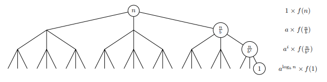
The Master Theorem provides a way to solve recurrence relations in which recursive calls decrease problem size by a constant factor.
Given a recurrence relation of the form $T(n) = aT(n/b)+ f(n)$ and $T(1) = Θ(1)$, with branching factor $a ≥ 1$, problem size reduction factor $b > 1$, and asymptotically non-negative function $f(n)$, the Master Theorem gives the solution to the recurrence by comparing $f(n)$ to $a^{log_b^{n}}=n^{log_b^a}$ , the number of leaves at the bottom of the recursion tree.
When $f(n)$ grows asymptotically faster than $n$ , the work done at each level decreases geometrically so the work at the root dominates;
alternatively, when $f(n)$ grows slower, the work done at each level increases geometrically and the work at the leaves dominates.
When their growth rates are comparable, the work is evenly spread over the tree’s $O(log n)$ levels.

tree

case	solution	conditions
1	$T(n) = \Theta(n^{log_b^a})$	$f(n) = \Theta(n^{log_b^{a-\epsilon}})$ for some constant $ε > 0$
2	$T(n) = \Theta(n^{log_b^a}log^{k+1}n)$	$T(n) = \Theta(n^{log_b^a}log^{k}n)$ for some constant $k ≥ 0$
3	$T(n) = \Theta(f(n))$	$f(n) = \Theta(n^{log_b^{a+\epsilon}})$ for some constant $ε > 0$ and $af(n/b) < cf(n)$ for some constant $0 < c < 1$

The Master Theorem takes on a simpler form when f(n) is a polynomial, such that the recurrence has the from $T(n) = aT(n/b) + Θ(n^c )$ for some constant $c ≥ 0$.

case	solution	conditions	intuition
1	$T(n) = \Theta(n^{log_b^a})$	$c < log_b^a$	Work done at leaves dominates
2	$T(n) = \Theta(n^{c}log^{n})$	$c=log_b^a$	Work balanced across the tree
3	$T(n) = \Theta(n^c)$	$c>log_b^a$	Work done at root dominates

This special case is straight-forward to prove by substitution (this can be done in recitation).
To apply the Master Theorem (or this simpler special case), you should state which case applies, and show that your recurrence relation satisfies all conditions required by the relevant case.
There are even stronger (more general) formulas to solve recurrences, but we will not use them in this class.

4 Hashing

Notes

Comparison Model

In this model, assume algorithm can only differentiate items via comparisons
Comparable items: black boxes only supporting comparisons between pairs
Comparisons are $<, ≤, >, ≥, =, \neq$, outputs are binary: True or False
Goal: Store a set of n comparable items, support find(k) operation
Running time is lower bounded by # comparisons performed, so count comparisons!

Decision Tree

Any algorithm can be viewed as a decision tree of operations performed
An internal node represents a binary comparison, branching either True or False
For a comparison algorithm, the decision tree is binary (draw example)
A leaf represents algorithm termination, resulting in an algorithm output
A root-to-leaf path represents an execution of the algorithm on some input
Need at least one leaf for each algorithm output, so search requires $≥ n + 1$ leaves

Comparison Search Lower Bound

What is worst-case running time of a comparison search algorithm?
running time $≥$ # comparisons $≥$ max length of any root-to-leaf path $≥$ height of tree
What is minimum height of any binary tree on $≥ n$ nodes?
Minimum height when binary tree is complete (all rows full except last)
$Height ≥ \lceil lg(n + 1) \rceil - 1 = Ω(log n)$, so running time of any comparison sort is $Ω(log n)$S
Sorted arrays achieve this bound! Yay!
More generally, height of tree with $Θ(n)$ leaves and max branching factor $b$ is $Ω(logb n)$
To get faster, need an operation that allows super-constant $ω(1)$ branching factor. How??

Direct Access Array

Exploit Word-RAM $O(1)$ time random access indexing! Linear branching factor!
Idea! Give item unique integer key k in $\{0, . . . , u - 1\}$, store item in an array at index $k$
Associate a meaning with each index of array.
If keys fit in a machine word, i.e. $u ≤ 2^w$, worst-case $O(1)$ find/dynamic operations! Yay!
6.006: assume input numbers/strings fit in a word, unless length explicitly parameterized
Anything in computer memory is a binary integer, or use (static) 64-bit address in memory
But space $O(u)$, so really bad if $n \ll u$ … :(
Example: if keys are ten-letter names, for one bit per name, requires $26^{10} ≈ 17.6$ TB space
How can we use less space?

Hashing

Idea! If $n \ll u$, map keys to a smaller range $m = Θ(n)$ and use smaller direct access array
Hash function: $h(k) : \{0, . . . , u - 1\} → \{0, . . . , m - 1\}$ (also hash map)
Direct access array called hash table, $h(k)$ called the hash of key k
If $m \ll u$, no hash function is injective by pigeonhole principle
Always exists keys $a, b$ such that $h(a) = h(b)$ $→$ Collision! :(
Can’t store both items at same index, so where to store? Either:
- store somewhere else in the array (open addressing)
  - complicated analysis, but common and practical
- store in another data structure supporting dynamic set interface (chaining)

Chaining

Idea! Store collisions in another data structure (a chain)
If keys roughly evenly distributed over indices, chain size is $n/m = n/Ω(n) = O(1)!$
If chain has $O(1)$ size, all operations take $O(1)$ time! Yay!
If not, many items may map to same location, e.g. $h(k) = constant$, chain size is $Θ(n)$ :(
Need good hash function! So what’s a good hash function?

Hash Functions

Division (bad): $h(k) = k \ \mod \ m$

Heuristic, good when keys are uniformly distributed!
$m$ should avoid symmetries of the stored keys
Large primes far from powers of 2 and 10 can be reasonable
Python uses a version of this with some additional mixing
If $u \ll n$, every hash function will have some input set that will a create $O(n)$ size chain
Idea! Don’t use a fixed hash function! Choose one randomly (but carefully)!

Universal (good, theoretically): $h_{ab}{(k)}=(((ak+b) \mod \ p) \mod \ m)$

Hash Family $$\mathcal{H}(p,m) = {h_{ab} a,b \in {0,…,p-1} and a \neq 0 }$$
Parameterized by a fixed prime $p > u$, with $a$ and $b$ chosen from range $\{0,...,p-1\}$
$\mathcal{H}$ is a Universal family: $\underset{h\in\mathcal{H}}{Pr}\{h(k_i) = h(k_j)\} \leq 1/m \qquad \forall k_i \neq k_j \in \{0,...,u-1\}$
Why is universality useful? Implies short chain lengths! (in expectation)
$X_{ij}$ indicator random variable over $h \in \mathcal{H}: \ X_{ij}=1 \ if \ h(k_i) = h(k_j), X_{ij} = 0 \ otherwise$
Size of chain at index $h(k_i)$ is random variable $X_i = \Sigma_{j}{X_{ij}}$
Expected size of chain at index $h(k_i)$:

\[\begin{align}\underset{h\in\mathcal{H}}{\mathbb{E}}{X_i} = \underset{h\in\mathcal{H}}{\mathbb{E}} \{\Sigma_{j}{X_{ij}}\} = \Sigma_{j}\underset{h\in\mathcal{H}}{\mathbb{E}}{X_{ij}} & = 1 + \Sigma_{j\neq i}\underset{h\in\mathcal{H}}{\mathbb{E}}{X_{ij}}\\ &= 1 + \Sigma_{j\neq i}(1)\underset{h\in\mathcal{H}}{Pr}\{h(k_i) = h(k_j)\} + (0)\underset{h\in\mathcal{H}}{Pr}\{h(k_i) \neq h(k_j)\}\\ &\leq 1 + \Sigma_{j\neq i} 1/m = 1 + (n-1) /m\end{align}\]

Since $m = Ω(n)$, load factor $α = n/m = O(1)$, so $O(1)$ in expectation!

Dynamic

If $n/m$ far from 1, rebuild with new randomly chosen hash function for new size m
Same analysis as dynamic arrays, cost can be amortized over many dynamic operations
So a hash table can implement dynamic set operations in expected amortized O(1) time! :)

Data Structure	API Type			Worst Case $O(\cdot)$
Set	Container	Static	Dynamic
API	`build(x)`	`find(k)`	`insert(k)` `delete(k)`	`find_min()` `find_max()`	`find_prev(k)` `find_next(k)`
Array	$n$	$n$	$n$	$n$	$n$
Sorted Array	$nlogn$	$logn$	$n$	$1$	$logn$
Direct Access Array	$u$	$1$	$1$	$u$	$u$
Hash Table	$n_{(e)}$	$1_{e}$	$1_{(a)(e)}$	$n$	$n$

5 Linear Sorting

Notes

Comparison Sort Lower Bound

Comparison model implies that algorithm decision tree is binary (constant branching factor)
Requires # leaves L ≥ # possible outputs
Tree height lower bounded by $Ω(log L)$, so worst-case running time is $Ω(log L)$
To sort array of n elements, # outputs is n! permutations
Thus height lower bounded by $log(n!) ≥ log((n/2)^{n/2}) = Ω(n log n) $
So merge sort is optimal in comparison model
Can we exploit a direct access array to sort faster?

Direct Access Array Sort

Example: $[5, 2, 7, 0, 4]$
Suppose all keys are unique non-negative integers in range ${0, . . . , u - 1}$, so $n ≤ u$
Insert each item into a direct access array with size $u$ in $Θ(n)$
Return items in order they appear in direct access array in $Θ(u)$
Running time is $Θ(u)$, which is $Θ(n)$ if $u = Θ(n)$. Yay!

def direct_access_sort(A):
    """Sort A assuming items have distinct non-negative keys."""
    u = 1 + max([x.key for x in A])
    D = [None] * u
    for x in A:
        D[x.key] = x
    i = 0
    for key in range(u):
        if D[key] is not None:
            A[i] = D[key]
            i += 1

What if keys are in larger range, like $u = Ω(n^2) < n^2$?
Idea! Represent each key $k$ by tuple $(a, b)$ where $k = an + b$ and $0 ≤ b < n$
Specifically $a = \lfloor k/n\rfloor < n$ and $b = (k \mod n)$ (just a 2-digit base-n number!)
This is a built-in Python operation $(a, b) = divmod(k, n)$
Example: $[17, 3, 24, 22, 12] ⇒ [(3,2), (0,3), (4,4), (4,2), (2,2)] ⇒ [32, 03, 44, 42, 22]_{(n=5)}$
How can we sort tuples?

Tuple Sort

Item keys are tuples of equal length, i.e. item $x.key = (x.k_1, x.k_2, x.k_3, . . .)$.
Want to sort on all entries lexicographically, so first key $k_1$ is most significant
How to sort? Idea! Use other auxiliary sorting algorithms to separately sort each key
(Like sorting rows in a spreadsheet by multiple columns)
What order to sort them in? Least significant to most significant!
Exercise: $[32, 03, 44, 42, 22] =⇒ [42, 22, 32, 03, 44] =⇒ [03, 22, 32, 42, 44]_{(n=5)}$
Idea! Use tuple sort with auxiliary direct access array sort to sort tuples (a, b).
Problem! Many integers could have the same a or b value, even if input keys distinct
Need sort allowing repeated keys which preserves input order
Want sort to be stable: repeated keys appear in output in same order as input
Direct access array sort cannot even sort arrays having repeated keys!
Can we modify direct access array sort to admit multiple keys in a way that is stable?

Counting Sort

Instead of storing a single item at each array index, store a chain, just like hashing!
For stability, chain data structure should remember the order in which items were added
Use a sequence data structure which maintains insertion order
To insert item x, insert_last to end of the chain at index $x.key$
Then to sort, read through all chains in sequence order, returning items one by one

def counting_sort(A):
    """Sort A assuming items have non-negative keys."""
    u = 1 + max([x.key for x in A])
    D = [[] for i in range(u)]
    for x in A:
        D[x.key].append(x)
    i = 0
    for chain in D:
        for x in chain:
            A[i] = x
            i += 1

Radix Sort

Idea! If $u < n^2$, use tuple sort with auxiliary counting sort to sort tuples (a, b)
Sort least significant key b, then most significant key a
Stability ensures previous sorts stay sorted
Running time for this algorithm is $O(2n) = O(n)$. Yay!
If every $key < n^c$ for some positive $c = logn(u)$, every key has at most $c$ digits base $n$
A c-digit number can be written as a c-element tuple in $O(c)$ time
We sort each of the c base-n digits in $O(n)$ time
So tuple sort with auxiliary counting sort runs in $O(cn)$ time in total
If c is constant, so each key is $≤ n^c$ , this sort is linear $O(n)$!

def radix_sort(A):
    """Sort A assuming items have non-negative keys"""
    n = len(A)
    u = 1 + max([x.key for x in A])
    c = 1 + (u.bit_length() // n.bit_length())
    
    class Obj: pass
    
    D = [Obj() for a in A]
    for i in range(n):
        D[i].digits = []
        D[i].item = A[i]
        high = A[i].key
        for j in range(c):
            high, low = divmod(high, n)
            D[i].digits.append(low)
	for i in range(c):
        for j in range(n):
            D[j].key = D[j].digits[i]
        counting_sort(D)
    for i in range(n);
    	A[i] = D[i].item

Algorithm	Time $O(\cdot)$	In-place?	Stable?	Comments
Insertion Sort	$n^2$	Y	Y	$O(nk)$ for k-proximate
Selection Sort	$n^2$	Y	N	$O(n)$ swaps
Merge Sort	$nlogn$	N	Y	stable, optimal comparison
Counting Sort	$n + u$	N	Y	$O(n)$ when $u = O(n)$
Radix Sort	$n + nlog_n{u}$	N	Y	$O(n)$ when $u = O(n)$

6 Binary Trees, Part 1

Notes

Sequence Data Structure	API Type			Worst Case $O(\cdot)$
Array	Container	Static	Dynamic
API	`build(x)`	`get_at(i)` `set_at(i)`	`insert_first(x)` `delete_first()`	`insert_last(x)` `delete_last()`	`insert_at(i, x)` `delete_at(i)`
Static Array	$n$	$1$	$n$	$n$	$n$
Linked List	$n$	$n$	$1$	$n$ # 1 if we keep track of tail	$n$
Dynamic Array	$n$	$1$	$n$	$1_{(a)}$	$n$
Goal	$n$	$logn$	$logn$	$logn$	$logn$

Set Data Structure	API Type			Worst Case $O(\cdot)$
Set	Container	Static	Dynamic
API	`build(x)`	`find(k)`	`insert(k)` `delete(k)`	`find_min()` `find_max()`	`find_prev(k)` `find_next(k)`
Array	$n$	$n$	$n$	$n$	$n$
Sorted Array	$nlogn$	$logn$	$n$	$1$	$logn$
Goal	$nlogn$	$logn$	$logn$	$logn$	$logn$

How? Binary Trees!

Pointer-based data structures (like Linked List) can achieve worst-case performance
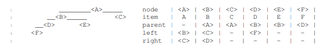
Binary tree is pointer-based data structure with three pointers per node
Node representation: node.{item, parent, left, right}
Example:

example tree

class TreeNode:
    def __init__(self, x):
        self.item = x
        self.left = None
        self.right = None
        self.parent = None

Terminology

The root of a tree has no parent (Ex: <A>)
leaf of a tree has no children (Ex: <C>,<E>, and <F>)
Define depth(<X>) of node <X> in a tree rooted at <A> to be length of path from <A> to <X>
Define height(<X>) of node <X> to be max depth of any node in the subtree rooted at <X>
Idea: Design operations to run in $O(h)$ time for root height $h$, and maintain $h = O(log n)$
A binary tree has an inherent order: its traversal order (In-order traversal)
- every node in node <X>’s left subtree is before <X>
- every node in node <X>’s right subtree is after <X>

def subtree_iter(A):
    if A.left: yield from A.left.subtree_iter()
    yield A
    if A.right: yield from A.right.subtree_iter()

List nodes in traversal order via a recursive algorithm starting at root:
- Recursively list left subtree, list self, then recursively list right subtree
- Runs in $O(n)$ time, since $O(1)$ work is done to list each node
- Example: Traversal order is (<F>,<D>,,<E>,<A>,<C>)
Right now, traversal order has no meaning relative to the stored items
Later, assign semantic meaning to traversal order to implement Sequence/Set interfaces

Find first node in the traversal order of node <X>’s subtree (last is symmetric)
- Otherwise, <X> is the first node, so return it
- Running time is $O(h)$ where h is the height of the tree
- Example: first node in <A>’s subtree is <F>

def subtree_first(A):
    if A.left: return A.left.subtree_first()
    return A

def subtree_last(A):
    if A.right: return A.right.subtree_last()
    return A

Find successor of node <X> in the traversal order (predecessor is symmetric)
- If <X> has right child, return first of right subtree
- Otherwise, return lowest ancestor of <X> for which <X> is in its left subtree
- Running time is $O(h)$ where $h$ is the height of the tree
- Example: Successor of:  is <E>, <E> is <A>, and <C> is None.

def successor(A):
    if A.right: return A.right.subtree_first()
    while A.parent and (A is A.parent.right):
        A = A.parent
	return A.parent

def predecessor(A):
    if A.left: return A.left.subtree_last()
    while A.parent and (A is A.parent.left):
        A = A.parent
    return A.parent

Dynamic Operations

Change the tree by a single item (only add or remove leaves):
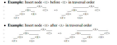
- add a node after another in the traversal order (before is symmetric)
- remove an item from the tree
Insert node <Y> after <X> in the traversal order
- If <X> has no right child, make <Y> the right child of <X>
- Otherwise, make <Y> the left child of <X>’s successor (which cannot have a left child)
- Running time is $O(h)$ where $h$ is the height of the tree

add_node

def subtree_insert_before(A, B):
    if A.left:
        A = A.left.subtree_last()
        A.right, B.parent = B, A
    else:
        A.left, B.parent = B, A
        
def subtree_insert_after(A, B):
    if A.right:
        A = A.right.subtree_first()
        A.left, B.parent = B, A
    else:
        A.right, B.parent = B, A

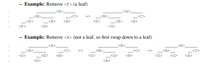
Delete the item in node <X> from <X>’s subtree
- If <X> is a leaf, detach from parent and return
- Otherwise, <X> has a child
 - If <X> has a left child, swap items with the predecessor of <X> and recurse
 - Otherwise <X> has a right child, swap items with the successor of <X> and recurse
- Running time is $O(h)$ where $h$ is the height of the tree

delete_node

def subtree_delete(A):
    if A.left or A.right:   # A is a leaf node
        if A.left: B = A.predecessor()
        else:      B = A.successor()
        A.item, B.item = B.item, A.item
    if A.parent:            # A is not a leaf node
        if A.parent.left is A: A.parent.left = None
        else:                  A.parent.right = None
	return A

Application: Set

Idea! Set Binary Tree (a.k.a Binary Search Tree / BST)
Traversal order(In-order) is sorted order increasing by key
- Equivalent to BST Property: for every node, every key in left subtree $\leq$ node’s key $\leq$ every key in right subtree
Then can find the node with key $k$ in node <X>’s subtree in $O(h)$ time like binary search:
- If $k$ is smaller than the key at <X>, recurse in left subtree (or return None)
- If $k$ is larger than the key at <X>, recurse in right subtree (or return None)
- Otherwise, return the item stored at <X>
Other Set operations follow a similar pattern

class BSTNode(TreeNode):
    def subtree_find(A, k):
        if k == A.item.key: return A
        if k < A.item.key and A.left: return A.left.subtree_find(k)
        if k > A.item.key and A.right: return A.right.subtree_find(k)
        
    def subtree_find_next(A, k):
        if A.item.key <= k:
            if A.right: return A.right.subtree_find_next(k)
            else:       return None
        if A.item.key > k:
            if A.left:
				B = A.left.subtree_find_next(k)
                if B: return B
        return A
    
    def subtree_find_prev(A, k):
        if A.item.key >= k:
            if A.left: return A.left.subtree_find_prev(k)
            else:      return None
            
        if A.item.key < k:
            if A.right:
                B = A.right.subtree_find_prev(k)
                if B: return B
		return A

    def subtree_insert(A, B):
        if B.item.key < A.item.key:
            if A.left: A.left.subtree_insert(B)
			else:      A.subtree_insert_before(B)
		elif B.item.key > A.item.key:
            if A.right: A.right.subtree_insert(B)
            else:       A.subtree_insert_after(B)
		else: A.item = B.item

class BinaryTree:
    def __init__(self, node_type=BinaryNode):
        self.root = None
        self.size = 0
        self.node_type = node_type
    
    def __len__(self): return self.size
    def __iter__(self): 
        if self.root:
            for item in self.root.subtree_iter():
                yield node.item
            
class BinaryTreeSet(BinaryTree):
    def __init__(self): 
        super().__init__(node_type=BSTNode)
	
    def iter_order(self): yield from self
	
    def build(self, X):
        for x in X: self.insert(x)
            
	def find_min(self):
        if self.root: return self.root.subtree_first().item
        
    def find_max(self):
        if self.root: return self.root_subtree_last().item
        
    def find(self, k):
        if self.root:
            node = self.root.subtree_find(k)
            if node: return node.item
            
	def find_next(self, k):
        if self.root:
            node = self.root.subtree_find_next(k)
            if node: return node.item
            
	def find_prev(self, k):
        if self.root:
            node = self.root.subtree_find_prev(k)
            if node: return node.item
	
    def insert(self, x):
        new_node = self.node_type(x)
        if self.root:
            self.root.subtree_insert(new_node)
            if new_node.parent is None: return False
        else:
            self.root = new_node
		self.size += 1
        
	def delete(self, k):
        assert self.root
        node = self.root.subtree_find(k)
        assert node
        ext = node.subtree_delete()
        if ext.parent is None: self.root = None
		self.size -= 1
		return ext.item

Application: Sequence

Idea! Sequence Binary Tree: Traversal order is sequence order
How do we find $i^th$ node in traversal order of a subtree? Call this operation subtree_at(i)
Could just iterate through entire traversal order, but that’s bad, $O(n)$
However, if we could compute a subtree’s size in $O(1)$, then can solve in $O(h)$ time
- How? Check the size $n_L$ of the left subtree and compare to $i$
- If $i < n_L$, recurse on the left subtree
- If $i > n_L$, recurse on the right subtree with $i’ = i - n_L - 1$
- Otherwise, $i = n_L$, and you’ve reached the desired node!
Maintain the size of each node’s subtree at the node via augmentation
- Add node.size field to each node
- When adding new leaf, add $+1$ to a.size for all ancestors a in $O(h)$ time
- When deleting a leaf, add $-1$ to a.size for all ancestors a in $O(h)$ time
Sequence operations follow directly from a fast subtree_at(i) operation
Naively, build(X) takes $O(nh)$ time, but can be done in $O(n)$ time; see recitation

7 Binary Tree II: AVL

Notes

Height Balance

How to maintain height $h=O(logn)$ where $n$ is number of nodes in tree?
A binary tree that maintains $O(logn)$ height under dynamic operations is called balanced
- There are many balancing schemes (Red-Black Trees, Splay Trees, 2-3 Trees, …)
- First proposed balancing scheme was the AVL Tree(Adelson-Velsky and Landis, 1962)

Rotations

Need to reduce height of tree without changing its traversal order, so that we represent the same sequence of items.
How to change the structure of a tree, while preserving traversal order? Rotations!
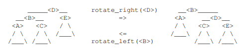
A rotation relinks $O(1)$ pointers to modify tree structure and maintains traversal order

def subtree_rotate_right(D):
    assert D.left
    B, E = D.left, D.right
    A, C = B.left, B.right
    
    # make sure new B has the right connection to D's parent
    D, B = B, D
    D.item, B.item = D.item, B.item
    
    B.left, B.right = A, D
    D.left, D.right = C, E
    
    if A: A.parent = B
    if E: E.parent = D
        
def subtree_rotate_left(B):
    assert B.right
    A, D = B.left, B.right
    C, E = D.left, D.right
    
    B, D = D, B
    B.item, D.item = D.item, B.item
    
    D.left, D.right = B, E
    B.left, B.right = A, C
    
    if A: A.parent = B
    if E: E.parent = D

Rotations Suffice

Claim: $O(n)$ rotations can transform a binary tree to any other with same traversal order
Proof: Repeatedly perform last possible right rotation in traversal order; resulting tree is a canonical chain. Each rotation increases depth of the last node by 1. Depth of last node in final chain is $n - 1$, so at most $n-1$ rotations are performed. Reverse canonical rotations to reach target tree. Q.E.D
Can maintain height-balance by using $O(n)$ rotations to fully balance the tree, but slow :(
We will keep the tree balanced in $O(logn)$ time per operation!

AVL Trees: Height Balance

AVL trees maintain height-balance (also called the AVL property)
- A node is height-balanced if heights of its left and right subtree differ by at most 1
- Let skew of a node be the height of its right subtree minus that of its left subtree
- Then a node is height-balanced if its skew is $-1,0$ or $1$
Claim: A binary tree with height-balanced nodes has height $h=O(logn)$ (i.e., $n=2^{\Omega(h)}$)
Proof: Suffices to show fewest nodes $F(h)$ in any height $h$ tree is $F(h)=2^{\Omega(h)}$ $F(0) = 1, F(1)=2, F(h)=1+F(h-1)+F(h-2)\geq 2F(h-2))\implies F(h)\geq 2^{h/2}\qquad \square$
Suppose adding or removing leaf from a height-balanced tree results in imbalance
- Only subtree of the leaf’s ancestors have changed in height or skew
- Heights changed by only $\pm 1$, so skews still have magnitude $\leq 2$
- Idea: Fix height-balance of ancestors starting from leaf up to the root
- Repeatedly rebalanced lowest ancestor that is not height-balanced, wlog assume skew 2
Local Rebalance: Given binary tree node :
- whose skew 2 and
- every other node in ’s subtree is height-balanced
- then ’s subtree can be made height-balanced via one or two rotations
- (after which <B?’s height is the same or one less than before)
Proof:
- Since skew of  is 2, ?’s right child exists
- Case 1: skew of <F> is 0 or Case 2: skew of <F> is 1
 - Perform a left rotation on

TBC

Computing Height

How to tell whether node is height-balanced? Compute heights of subtrees!
How to compute the height of node <X> ? Naive algorithm:
- Recursively compute height of the left and right subtrees of <X>
- Add $1$ to the max of the two heights
- Runs in $Ω(n)$ time, since we recurse on every node :(
Idea: Augment each node with the height of its subtree! (Save for later!)
Height of <X> can be computed in $O(1)$ time from the heights of its children:
- Look up the stored heights of left and right subtrees in $O(1)$ time
- Add $1$ to the max of the two heights
During dynamic operations, we must maintain our augmentation as the tree changes shape
Recompute subtree augmentations at every node whose subtree changes:
- Update relinked nodes in a rotation operation in $O(1)$ time (ancestors don’t change)
- Update all ancestors of an inserted or deleted node in $O(h)$ time by walking up the tree

Steps to Augment a Binary Tree

In general, to augment a binary tree with a subtree property P, you must:
- State the subtree property P(<X>) you want to store at each node <X>
- Show how to compute P(<X>) from the augmentations of <X>’s children in $O(1)$ time
- Then stored property P(<X>) can be maintained without changing dynamic operation costs

Application: Sequence

For sequence binary tree, we needed to know subtree sizes
For just inserting/deleting a leaf, this was easy, but now need to handle rotations
Subtree size is a subtree property, so can maintain via augmentation
- Can compute size from sizes of children by summing them and adding 1

Conclusion

Set AVL trees achieve $O(log n)$ time for all set operations
except $O(n log n)$ time for build and $O(n)$ time for iter
Sequence AVL trees achieve $O(log n)$ time for all sequence operations
except $O(n)$ time for build and iter

Application: Sorting

Any Set data structure defines a sorting algorithm: build (or repeatedly insert) then iter
For example, Direct Access Array Sort from Lecture 5
AVL Sort is a new $O(n log n)$ time sorting algorithm

8 Binary Heaps

Notes

Priority Queue Interface

Keep track of many items, quickly access/remove the most important
- Example: router with limited bandwidth, must prioritize certain kinds of messages
- Example: process scheduling in operating system kernels
- Example: discrete-event simulation (when is next occurring event?)
- Example: graph algorithms (later in the course)
Order items by key = priority so Set interface (not Sequence interface)

Optimized for a particular subset of Set operations:

Operation	Specification
`build(X)`	build priority queue from iterable X
`insert(x)`	add item x to data structure
`delete_max()`	remove and return stored item with largest key
`find_max()`	return stored item with largest key

(Usually optimized for max or min, not both)
Focus on insert and delete_max operations: build can repeatedly insert; find_max() can insert(delete_min())

class PriorityQueue:
    def __init__(self):
        self.A = []
    
    def insert(self, x):
        self.A.append(x)
        
    def delete_max(self):
        assert len(self.A) > 0
        return self.A.pop()   # not correct by it self.
    
    @classmethod
    def sort(PQ, A):
        pq = PQ()
        for x in A: pq.insert(x)
        out = [pq.delete_max() for _ in A]
        return reversed(out) 

Priority Queue Sort

Any priority queue data structure translates into a sorting algorithm:
- build(A), e.g., insert items one by one in input order
- Repeatedly delete_min() (or delete_max()) to determine (reverse) sorted order
All the hard work happens inside the data structure
Running time is $T_{build} + n · T_{delete_max} ≤ n · T_{insert} + n · T_{delete_max}$
Many sorting algorithms we’ve seen can be viewed as priority queue sort:

Priority Queue Data Structure		Operations $O(\cdot)$		Priority Queue Sort		Algorithm
	`build(A)`	`insert(x)`	`delete_max()`	Time	In-place?
Dynamic Array	$n$	$1_{(a)}$	$n$	$n^2$	Y	Selection Sort
Sorted Dynamic Array	$nlogn$	$n$	$1_{(a)}$	$n^2$	Y	Insertion Sort
Set AVL Tree	$nlogn$	$logn$	$logn$	$nlogn$	N	AVL Sort
Goal	$n$	$logn_{(a)}$	$logn_{(a)}$	$nlogn$	Y	Heap Sort

Priority Queue: Set AVL Tree

Set AVL trees support insert(x), find_min(), find_max(), delete_min(), and delete_max() in $O(log n)$ time per operation
So priority queue sort runs in $O(n log n)$ time
- This is (essentially) AVL sort from Lecture 7
Can speed up find_min() and find_max() to $O(1)$ time via subtree augmentation
But this data structure is complicated and resulting sort is not in-place
Is there a simpler data structure for just priority queue, and in-place $O(n lg n)$ sort? YES, binary heap and heap sort
Essentially implement a Set data structure on top of a Sequence data structure (array), using what we learned about binary trees

Priority Queue: Array

Store elements in an unordered dynamic array
insert(x): append x to end in amortized $O(1)$ time
delete_max(): find max in $O(n)$, swap max to the end an d remove
insert is quick, but delete_max is slow
Priority queue sort is selection sort! (plus some copying)

class PQArray(PriorityQueue):
    def delete_max(self):  # O(n)
        n, A, m = len(self.A), self.A, 0
        for i in range(1, n):
            m = i if A[m].key < A[i].key else m
        A[m], A[n] = A[n], A[m]
        return super().delete_max()  # pop from end

We use *args to allow insert to take one argument (as makes sense now) or zero arguments; we will need the latter functionality when making the priority queues in-place.

Priority Queue: Sorted Array

Store elements in a sorted dynamic array
insert(x): append x to end, swap down to sorted position in $O(n)$ time
` delete_max()`: delete from end in $O(1)$ amortized
delete_max is quick, but insert is slow
Priority queue sort is insertion sort! (plus some copying)
Can we find a compromise between these two array priority queue extremes?

class PQSortedArray(PriorityQueue):
    def insert(self, x=None):
        if x is not None: super().insert(x)
        i, A = len(self.A) - 1, self.A
        while 0 < i and A[i+1].key < A[i].key:
            A[i+1], A[i] = A[i], A[i+1]
           	i -= 1

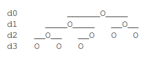
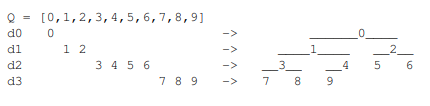
Array as a Complete Binary Tree

Idea: interpret an array as a complete binary tree, with maximum $2^i$ nodes at depth $i$ except at the largest depth, where all nodes are left-aligned
Equivalently, complete tree is filled densely in reading order: root to leaves, left to right
Perspective: bijection between arrays and complete binary trees
Height of complete tree perspective of array of $n$ item is $\lceil log n \rceil$, so balanced binary tree

tree

Implicit Complete Tree

Complete binary tree structure can be implicit instead of storing pointers
Root is at index 0
Compute neighbors by index arithmetic:

\[\begin{align} left(i) &=2i+1 \\ right(i) &=2i+2 \\ parent(i) &= \lfloor \frac{i-1}{2} \rfloor \end{align}\]

Binary Heaps

Idea: keep larger elements higher in tree, but only locally
Max-Heap Property at node $i: Q[i] ≥ Q[j] for j ∈ {left(i),right(i)}$
Max-heap is an array satisfying max-heap property at all nodes
Claim: In a max-heap, every node i satisfies $Q[i] ≥ Q[j]$ for all nodes $j$ in subtree(i)
Proof:
- Induction on $d = depth(j) - depth(i)$
- Base case: $d = 0$ implies $i = j$ implies $Q[i] ≥ Q[j]$ (in fact, equal)
- $depth(parent(j)) - depth(i) = d - 1 < d$, so $Q[i] ≥ Q[parent(j)]$ by induction
- $Q[parent(j)] ≥ Q[j]$ by Max-Heap Property at parent(j)
In particular, max item is at root of max-heap

def parent(i):
    p = (i - 1) // 2
    return p if 0 < i else i

def left(i, n):
    l = 2 * i + 1
    return l if l < n else i

def right(i, n):
    r = 2 * i + 2
    return r if r < n else i

Heap Insert

Append new item $x$ to end of array in $O(1)$ amortized, making it next leaf $i$ in reading order
max_heapify_up(i): swap with parent until Max-Heap Property
- Check whether $Q[parent(i)] \geq Q[i]$ (part of Max-Heap Property at parent(i))
- If not, swap items $Q[i]$ and $Q[parent(i)]$, and recursively max_heapify_up(parent(i))
Correctness:
- Max-Heap Property guarantees all nodes $\geq$ descendants, except $Q[i]$ might be > some of its ancestors (unless $i$ is the root, so we’re done)
- If swap is necessary, same guarantee is true with $Q[parent(i)]$ instead of $Q[i]$
Running time: height of tree, so $\Theta(\log n)$

Heap Delete Max

Can only easily remote last element from dynamic array, but max key is in root of tree
So swap item at root node $i = 0$ with last item at node $n-1$ in heap array
max_heapify_down(i): swap root with larger child until Max-Heap Property
- Check whether $Q[i] \geq Q[j] \ for \ j \in {left(i), right(i)}$ (Max-Heap Property at i)
- If not, swap $Q[i]$ with $Q[j]$ for child $j \ \in {left(i), right(i)}$ with maximum key, and recursively max_heapify_down(j)
Correctness:
- Max-Heap Property guarantees all nodes $\geq$ descendants, except $Q[i]$ might be < some descendants (unless $i$ is a leaf, so we’re done)
- If swap is necessary, same guarantee is true with $Q[j]$ instead of $Q[i]$
Running time: height of tree, so $\Theta(\log n)$

class PQHeap(PriorityQueue):
    def insert(self, x=None):
        if x: super().insert(x)
		n, A = self.n, self.A
        max_heapify_up(A, n, n-1)
    
    def delete_max(self):
        n, A = self.n, self.A
        A[0], A[n] = A[n], A[0]
        max_heapify_down(A, n, 0)
        return super().delete_max()
    
def max_heapify_up(A, n, c):
    p = parent(c)
    if A[p].key < A[c].key:
        A[c], A[p] = A[p], A[c]
        max_heapify_up(A, n, p)
        
        
def max_heapify_down(A, n, p):
    l, r = left(p, n), right(p, n)
    c = l if A[r].key < A[l].key else r
    if A[p].key < A[c].key:
        A[c], A[p] = A[p], A[c]
        max_heapify_down(A, n, c)    

Heap Sort

Plugging max-heap into priority queue sort gives us a new sorting algorithm
Running time is $O(n log n)$ because each insert and delete_max takes $O(log n)$
But often include two improvements to this sorting algorithm:

In-place Priority Queue Sort

Max-heap $Q$ is a prefix of a larger array $A$, remember how many items $ Q $ belong to heap
$ Q $ is initially zero, eventually $ A $ (after inserts), then zero again (after deletes)
insert() absorbs next item in array at index $ Q $ into heap
delete_max() moves max item to end, then abandons it by decrementing $ Q $
In-place priority queue sort with Array is exactly Selection Sort
In-place priority queue sort with Sorted Array is exactly Insertion Sort
In-place priority queue sort with binary Max Heap is Heap Sort

class PriorityQueue:
    def __init__(self, A):
        self.n, self.A = 0, A
    
    def insert(self):
        assert self.n < len(self.A)
        self.n += 1
    
    def delete_max(self):
        assert self.n >= 1
        self.n -= 1
    
    @classmethod
    def sort(Queue, A):
        pq = Queue(A)
        for i in range(len(A)): pq.insert()
        for i in range(len(A)): pq.delete_max()
        return pq.A

Linear Build Heap

Inserting $n$ items into heap call max_heapify_up(i) for $i$ from $0$ to $n-1$ (root down): $worst-case \ swaps \approx \Sigma_{i=0}^{n-1}depth(i)=\Sigma_{i=0}^{n-1}logi=log(n!)\geq(n/2)log(n/2)=\Omega(nlogn)$
Idea! Treat full array as a complete binary tree from start, then max_heapify_down(i) for i from $n-1$to $0$ (leaves up): $worst-case \ swaps \approx \Sigma_{i=0}^{n-1}height(i)=\Sigma_{i=0}^{n-1}(logn -logi)=log(\frac{n^n}{n!})=\Theta(log(\frac{n^n}{\sqrt{n}(n/e)^n}))=O(n)$
So can build heap in $O(n)$ time
(Doesn’t speed up $O(nlogn)$ performance of heap sort)

def build_max_heap(A):
    n = len(A)
    for i in range(n // 2, -1, -1):
        max_heapify_down(A, n, i)

Sequence AVL Tree Priority Queue

Where else have we seen linear build time for an otherwise logarithmic data structure? Sequence AVL Tree!
Store items of priority queue in Sequence AVL Tree in arbitrary order (insertion order)
Maintain max (and/or min) augmentation:
- node.max = pointer to node in subtree of node with maximum key
  - This is a subtree property, so constant factor overhead to maintain
find_min() and find _max() in $O(1)$ time
delete_min() and delete_max() in $O(log n)$ time
build(A) in $O(n)$ time
Same bounds as binary heaps (and more)

Set vs. Multiset

While our Set interface assumes no duplicate keys, we can use these Sets to implement Multisets that allow items with duplicate keys:
- Each item in the Set is a Sequence (e.g., linked list) storing the Multiset items with the same key, which is the key of the Sequence
In fact, without this reduction, binary heaps and AVL trees work directly for duplicate-key items (where e.g. delete_max deletes some item of maximum key), taking care to use ≤ constraints (instead of < in Set AVL Trees)

9 Breadth-First Search

Notes

Graph Applications

Why? Graphs are everywhere!
any network system has direct connection to graphs
e.g., road networks, computer networks, social networks
the state space of any discrete system can be represented by a transition graph
e.g., puzzle & games like Chess, Tetris, Rubik’s cube
e.g., application workflows, specifications

Graph Definitions

graph

Graph $G = (V, E)$ is a set of vertices $V$ and a set of pairs of vertices $E \subseteq V \times X$
Directed edges are ordered pairs, e.g., $(u, v)$ for $u, v \in V$
Undirected edges are unordered pairs, ${u, v}$ for $u, v \in V$ i.e., $(u, v)$ and $(v, u)$
In this class, we assume all graphs are simple:
- edges are distinct, e.g., $(u, v)$ only occurs once in E (though $(v, u)$ may appear), and
- edges are pairs of distinct vertices, e.g., $u \neq v$ for all $(u, v) ∈ E$
- Simple implies $\vert E \vert = O(\vert V \vert ^2)$, since $\vert E \vert ≤ \big(\frac{\vert V \vert }{2}\big)$for undirected, $≤ 2 \big(\frac{\vert V \vert }{2}\big)$ for directed

Neighbor Sets/Adjacencies

The outgoing neighbor set of $u ∈ V$ is $Adj^+(u) = {v ∈ V (u, v) ∈ E} $
The incoming neighbor set of $u ∈ V$ is $Adj^-(u) = {v ∈ V (v, u) ∈ E}$
The out-degree of a vertex $u ∈ V$ is $deg^+(u) = Adj^+(u) $
The in-degree of a vertex $u ∈ V$ is $deg^-(u) = Adj^-(u) $
For undirected graphs, $Adj^-(u) = Adj^+(u)$ and $deg^-(u) = deg^+(u)$
Dropping superscript defaults to outgoing, i.e., $Adj(u) = Adj^+(u)$ and $deg(u) = deg^+(u)$

Graph Representations

To store a graph $G = (V, E)$, we need to store the outgoing edges $Adj(u)$ for all $u ∈ V$
First, need a Set data structure $Adj$ to map $u$ to $Adj(u)$
Then for each $u$, need to store $Adj(u)$ in another data structure called an adjacency list
Common to use direct access array or hash table for $Adj$, since want lookup fast by vertex
Common to use array or linked list for each $Adj(u)$ since usually only iteration is needed
For the common representations, $Adj$ has size $Θ(\vert V \vert )$, while each $Adj(u)$ has size $Θ(deg(u))$
Since $\Sigma_{u∈V} deg(u) ≤ 2\vert E \vert $ by handshaking lemma, graph storable in $Θ( V + \vert E \vert ) $ space
Thus, for algorithms on graphs, linear time will mean $Θ( V + \vert E \vert )$ (linear in size of graph)

Paths

A path is a sequence of vertices $p = (v_1, v_2, . . . , v_k)$ where $(v_i, v_{i+1}) ∈ E$ for all $1 ≤ i < k$.
A path is simple if it does not repeat vertices
The length $\mathcal{l}(p)$ of a path $p$ is the number of edges in the path
The distance $δ(u, v)$ from $u ∈ V$ to $v ∈ V$ is the minimum length of any path from $u$ to $v$
- i.e., the length of a shortest path from $u$ to $v$
- (by convention, $δ(u, v) = ∞$ if $u$ is not connected to $v$)

Graph Path Problems

There are many problems you might want to solve concerning paths in a graph:
SINGLE_PAIR_REACHABILITY(G, s, t): is there a path in $G$ from $s ∈ V$ to $t ∈ V$ ?
SINGLE_PAIR_SHORTEST_PATH(G, s, t): return distance $δ(s,t)$, and a shortest path in $G = (V, E)$ from $s ∈ V$ to $t ∈ V$
SINGLE_SOURCE_SHORTEST_PATHS(G, s): return $δ(s, v)$ for all $v ∈ V$ , and a shortest-path tree containing a shortest path from $s$ to every $v ∈ V$ (defined below)
Each problem above is at least as hard as every problem above it (i.e., you can use a black-box that solves a lower problem to solve any higher problem)
We won’t show algorithms to solve all of these problems
Instead, show one algorithm that solves the hardest in $O( V + \vert E \vert )$ time!

Shortest Paths Tree

How to return a shortest path from source vertex $s$ for every vertex in graph?
Many paths could have length $Ω(\vert V \vert )$, so returning every path could require $Ω(\vert V \vert ^2) $ time
Instead, for all $v ∈ V$ , store its parent $P(v)$: second to last vertex on a shortest path from $s$
Let $P(s)$ be null (no second to last vertex on shortest path from $s$ to $s$)
Set of parents comprise a $shortest paths tree$ with $O(|V |)$ size! (i.e., reversed shortest paths back to $s$ from every vertex reachable from $s$)

Breadth-First Search (BFS)

How to compute $δ(s, v)$ and $P(v)$ for all $v ∈ V$ ?
Store $δ(s, v)$ and $P(v)$ in Set data structures mapping vertices $v$ to distance and parent
(If no path from $s$ to $v$, do not store $v$ in $P$ and set $δ(s, v)$ to $∞$)
Idea! Explore graph nodes in increasing order of distance
Goal: Compute level sets $L_i = {v v ∈ V and d(s, v) = i}$ (i.e., all vertices at distance $i$)
Claim: Every vertex $v ∈ L_i$ must be adjacent to a vertex $u ∈ L_{i-1}$ (i.e., $v ∈ Adj(u)$)
Claim: No vertex that is in $L_j$ for some $j < i$, appears in $L_i$
Invariant: $δ(s, v)$ and $P(v)$ have been computed correctly for all $v$ in any $L_j$ for $j < i$
Base case $(i = 1): L_0 = {s}, δ(s, s) = 0, P(s) = None$
Inductive Step: To compute $L_i$:
- for every vertex $u$ in $L_{i-1}$:
 - for every vertex $v ∈ Adj(u)$ that does not appear in any $L_j$ for $j < i$:
 - add $v$ to $L_i$, set $δ(s, v) = i$, and set $P(v) = u$
Repeatedly compute $L_i$ from $L_j$ for $j < i$ for increasing $i$ until $L_i$ is the empty set
Set $δ(s, v) = ∞$ for any $v ∈ V$ for which $δ(s, v)$ was not set
Breadth-first search correctly computes all $δ(s, v)$ and $P(v)$ by induction

Running time analysis:

Store each $L_i$ in data structure with $Θ(

L_i

)$ time iteration and $O(1)$ time insertion (i.e., in a dynamic array or linked list)

Checking for a vertex $v$ in any $L_j$ for $j < i$ can be done by checking for $v$ in $P$
Maintain $δ$ and $P$ in Set data structures supporting dictionary ops in $O(1)$ time (i.e., direct access array or hash table)
Algorithm adds each vertex $u$ to $≤ 1$ level and spends $O(1)$ time for each $v ∈ Adj(u)$
Work upper bounded by $O(1) × \Sigma_{u\in V} deg(u) = O(\vert E \vert )$ by handshake lemma
Spend $Θ( V )$ at end to assign $δ(s, v)$ for vertices $v ∈ V$ not reachable from $s$So
breadth-first search runs in linear time! $O( V + \vert E \vert ) $

def bfs(adj, s):
    parent = [None for v in adj]
    parent[s] = s
    levels = [[s]]
    while 0 < len(levels[-1]):
        level = []
        for u in levels[-1]:
            for v in adj[u]:
                if parent[v] is None:
                    parent[v] = u
                    level.append(v)
    	levels.append(level)
    return parents

def unweighted_shortest_path(adj, s, t):
    parents = bfs(adj, s)
    if parent[t] is None: return None
    i = t
    path = [t]
    while i != s:
        i = parent[i]
        path.append(i)
    return reversed(path)

10 Depth-First Search

Notes

Depth-First Search (DFS)

Searches a graph from a vertex $s$, similar to BFS
Solves Single Source Reachability, not Single Source Shortest Paths. Useful for solving other problems (later)!
Return (not necessarily shortest) parent tree of parent pointers back to $s$.
Idea! Visit outgoing adjacencies recursively, but never revisit a vertex
i.e., follow any path until you get stuck, backtrack until finding an unexplored path to explore
$P(s) = None$, then run $visit(s)$, where
visit(u)
- for every $v \in Adj(u)$ that does not appear in $P$:
  - set $P(v)= u$ and recursively call visit(v)
- (DFS finishes visiting vertex $u$, for use later!)

def dfs(adj, s, parent=None, order=None):
    if parent is None:
        parent = [None for v in adj]
        parent[s] = s
        order = []
    for v in adj[s]:
        if parent[v] is None:
            parent[v] = s
            dfs(adj, v, parent, order)
    order.append(s)
    return parent, order

Correctness

Claim: DFS visits $v$ and correctly sets $P(v)$ for every vertex $v$ reachable from $s$
Proof: induct on $k$, for claim on only vertices within distance $k$ from $s$
- Base case $(k = 0): P(s)$ is set correctly for $s$ and $s$ is visited
- Inductive step: Consider vertex $v$ with $δ(s, v) = k’ + 1$
- Consider vertex $u$, the second to last vertex on some shortest path from $s$ to $v$
- By induction, since $δ(s, u) = k’$ , DFS visits $u$ and sets $P(u)$ correctly
- While visiting $u$, DFS considers $v ∈ Adj(u)$
- Either $v$ is in $P$, so has already been visited, or $v$ will be visited while visiting $u$
- In either case, $v$ will be visited by DFS and will be added correctly to $P$ $\square$

Running Time

Algorithm visits each vertex $u$ at most once and spends $O(1)$ time for each $v ∈ Adj(u)$
Work upper bounded by $O(1) × \Sigma_{u \in V}deg(u) = O(\vert E \vert )$
Unlike BFS, not returning a distance for each vertex, so DFS runs in $O(\vert E \vert )$ time

Full-BFS and Full-DFS

Suppose want to explore entire graph, not just vertices reachable from one vertex
Idea! Repeat a graph search algorithm $A$ on any unvisited vertex
Repeat the following until all vertices have been visited:
- Choose an arbitrary unvisited vertex $s$, use $A$ to explore all vertices reachable from $s$
We call this algorithm Full-A, specifically Full-BFS or Full-DFS if A is BFS or DFS
Visits every vertex once, so both Full-BFS and Full-DFS run in $O(\vert V \vert + \vert E \vert )$ time

def full_dfs(adj):
    parent = [None for v in adj]
    order = []
    for v in range(len(adj)):
        if parent[v] is None:
            parent[v] = v
            dfs(adj, v, parent, order)
    return parent, order

DFS Edge Classification

Consider a graph edge from vertex $u$ to $v$, we call the edge a tree edge if the edge is part of the DFS tree (i.e. $parent[v] = u$)
Otherwise, the edge from $u$ to $v$ is not a tree edge, and is either:
- a back edge - $u$ is a descendant of $v$
- a forward edge - $v$ is a descendant of $u$
- a cross edge - neither are descendants of each other

Graph Connectivity

An undirected graph is connected if there is a path connecting every pair of vertices
In a directed graph, vertex $u$ may be reachable from $v$, but $v$ may not be reachable from $u$
Connectivity is more complicated for directed graphs (we won’t discuss in this class)
Connectivity(G): is undirected graph G connected?
Connected_Components(G): given undirected graph $G = (V, E)$, return partition of $V$ into subsets $V_i ⊆ V$ (connected components) where each $V_i$ is connected in $G$ and there are no edges between vertices from different connected components
Consider a graph algorithm $A$ that solves Single Source Reachability
Claim: $A$ can be used to solve Connected Components
Proof: Run Full-$A$. For each run of $A$, put visited vertices in a connected component $\square$

Topological Sort

A Directed Acyclic Graph (DAG) is a directed graph that contains no directed cycle
A Topological Order of a graph $G = (V, E)$ is an ordering $f$ on the vertices such that: every $edge (u, v) ∈ E$ satisfies $f(u) < f(v)$
Exercise: Prove that a directed graph admits a topological ordering if and only if it is a DAG
How to find a topological order?
A Finishing Order is the order in which a Full-DFS finishes visiting each vertex in G
Claim: If $G = (V, E)$ is a DAG, the reverse of a finishing order is a topological order
Proof: Need to prove, for every $edge (u, v) ∈ E$ that $u$ is ordered before $v$, i.e., the visit to $v$ finishes before visiting $u$. Two cases:
- If $u$ visited before $v$:
  - Before visit to $u$ finishes, will visit $v$ (via $(u, v)$ or otherwise)
  - Thus the visit to $v$ finishes before visiting $u$
- If $v$ visited before $u$:
  - $u$ can’t be reached from $v$ since graph is acyclic
  - Thus the visit to $v$ finishes before visiting $u$

Cycle Detection

Full-DFS will find a topological order if a graph $G = (V, E)$ is acyclic
If reverse finishing order for Full-DFS is not a topological order, then $G$ must contain a cycle
Check if $G$ is acyclic: for each edge $(u, v)$, check if $v$ is before $u$ in reverse finishing order
Can be done in $O(\vert E \vert )$ time via a hash table or direct access array
To return such a cycle, maintain the set of ancestors along the path back to $s$ in Full-DFS
Claim: If $G$ contains a cycle, Full-DFS will traverse an edge from $v$ to an ancestor of $v$
Proof: Consider a cycle $(v_0, v_1, . . . , v_k, v_0)$ in $G$
- Without loss of generality, let $v_0$ be the first vertex visited by Full-DFS on the cycle
- For each $v_i$, before visit to $v_i$ finishes, will visit $v_{i+1}$ and finish
- Will consider edge $(v_i, v_{i+1})$, and if $v_{i+1}$ has not been visited, it will be visited now
- Thus, before visit to $v_0$ finishes, will visit $v_k$ (for the first time, by $v_0$ assumption)
- So, before visit to $v_k$ finishes, will consider $(v_k, v_0)$, where $v_0$ is an ancestor of $v_k$ $\square$

11 Weighted Shortest Paths

Notes

Weighted Graphs

A weighted graph is a graph $G = (V, E)$ together with a weight function $w: E \rightarrow Z$
i.e., assign each edge $e = (u, v) \in E$ an integer weight: $w(e) = w(u, v)$
Many applications for edge weights in a graph:
- distances in road network
- latency in network connections
- strength of a relationship in a social network
Two common ways to represent weights computationlly:
- Inside graph representation: store edge weight with each vertex in adjacency lists
- Store separate Set data structure mapping each edge to its weight
We assume a representation that allows querying the weight of an edge in $O(1)$ time
Examples

Weighted Paths

The weight $w(\pi)$ of a path $\pi$ in a weighted graph is the sum of weights of edges in the path
The (weighted) shortest path from $s \in V$ to $t \in V$ is path of minimum weight from $s$ to $t$
$\delta(s, t) = inf{w(\pi) \ path \ \pi \ from \ s \ to \ t}$ is the shortest-path weight from $s$ to $t$
(Often use “distance” for shortest -path weight in weighted graphs, not number of edges)
As with unweighted graphs:
- $\delta(s,t) = \inf$ if no path from $s$ to $t$
- Subpaths of shortest paths are shortest paths (or else could splice in a shortest path)
Why infimum not minimum? Possible that no finite-length minimum-weight path exists
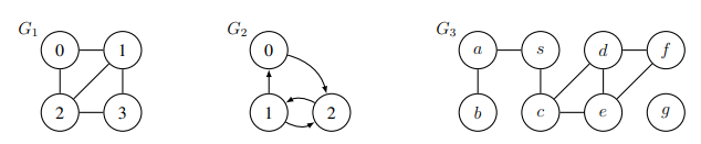
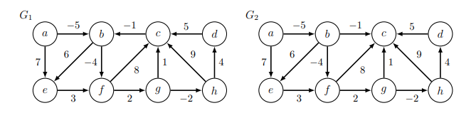
When? Can occur if there is a negative-weight cycle in the graph, Ex: $(b,f,g,c,b)$ in $G1$
A negative-weight cycle is a path $\pi$ starting and ending at same vertex $w(\pi) < 0$
$\delta (s, t) = - \infty$ if there is a path from $s$ to $t$ through a vertex on a negative-weight cycle
If this occurs, don’t want a shortest path, but may want the negative-weight cycle

Weighted Shortest Paths Algorithms

Already know one algorithm: Breadth-First Search! Runs in $O(\vert V \vert + \vert E \vert )$ time when, e.g.:
- graph has positive weights, and all weights are the same
- graph has positive weights, and sum of all weights at most $O(\vert V \vert + \vert E \vert )$
For general weighted graphs, we don’t know how to solve SSSP in $O(\vert V \vert + \vert E \vert )$ time
But if your graph is a Directed Acyclic Graph you can!

Restrictions		SSSP Algorithm
Graph	Weights	Name	Running Time $O(\cdot)$
General	Unweighted	BFS	$\vert V \vert + \vert E \vert $
DAG	Any	DAG Relaxation	$\vert V \vert + \vert E \vert $
General	Any	Bellman-Ford	$\vert V \vert \cdot\vert E \vert $
General	Non-negative	Dijkstra	$\vert V \vert log\vert V \vert + \vert E \vert $

Shortest-Paths Tree

For BFS, we kept track of parent pointers during search. Alternatively, compute them after!
If know $\delta(s, v)$ for all vertices $v\in V$, can construct shortest-path tree in $O(\vert V \vert + \vert E \vert )$ time
For weighted shortest paths from $s$, only need parent pointers for vertices $v$ with finite $\delta(s, v)$
Initialize empty $P$ and set $P(s) = None$
For each vertex $u\in V$ where $\delta(s, u)$ is finite:
- For each outgoing neighbor $v \in Adj^+(u)$:
  - If $P(v)$ not assigned and $\delta(s, v) = \delta(s, u) + w(u, v)$
    - There exits a shortest path through edge $(u, v)$, so set $P(v) = u$
Parent pointers may traverse cycles of zero weight. Mark each vertex in such a cycle.
For each unmarked vertex $u\in V$ (including vertices later marked):
- For each $v\in Adj^+(u)$ where $v$ is marked and $\delta(s, v) = \delta(s, u) + w(u, v)$
  - Unmark vertices in cycle containing $v$ by traversing parent pointers from $v$
  - Set $P(v) = u$, breaking the cycle

Relaxation

A relaxation algorithm searches for a solution to an optimization problem by starting with a solution that is not optimal, then iteratively improves the solution until it becomes an optimal solution to the original problem.

def try_to_relax(adj, w, d, parent, u, v):
    if d[v] > d[u] + w(u, v):
        d[v] = d[u] + w(u, v)
        parent[v] = u
        
def general_relax(adj, w, s):
    d = [float('inf') for _ in adj]
    parent = [None for _ in adj]
    d[s], parent[s] = 0, s
    while some_edge_relaxable(adj, w, d):
        (u, v) = get_relaxable_edge(adj, w, d)
        try_to_relax(adj, w, d, parent, u, v)
    return d, parent

DAG Relaxation

Idea! Maintain a distance estimate $d(s, v)$ (initially $\infty$ ) for each vertex $v\in V$, that always upper bounds true distance $\delta(s, v)$, then gradually lowers until $d(s, v) = \delta(s, v)$
When do we lower? When an edge violates the triangle inequality!
Triangle Inequality: the shortest-path weight from $u$ to $v$ cannot be greater than the shortest path from $u$ to $v$ through another vertex $x$, i.e., $\delta(u, v) \neq \delta(u, x) + \delta(x, v)$ for all $u, v, x \in V$
If $d(s, v) > d(s, u) + w(u, v)$ for some edge $u, v$, then triangle inequality is violated :(
Fix by lowering $d(s, v)$ to $d(s, u) + w(u, v)$, i.e., relax $(u, v)$ to satisfy violated constraint
Claim: Relaxation is safe: maintains that each $d(s, v)$ is weight of a path to $v$ (or $\infty$) $\forall v \in V$
Proof: Assume $d(s, v’)$ is weight of a path (or $\infty$) for $\forall v’ \in V$. Relaxing some edge $(u, v)$ sets $d(s, v)$ to $d(s, u) + w(u, v)$, which is the weight of a path from $s$ to $v$ through $u$ $\qquad \square$
Set $d(s, v) = \infty$ for all $v \in V$, then set $d(s, s) = 0$
Process each vertex $u$ in a topological sort order of G:
- For each outgoing neighbor $v \in Adj^+(u)$:
  - If $d(s, v) > d(s, u) + w(u, v)$
    - relax edge $(u, v)$, i.e., set $d(s, v) = d(s, u) + w(u, v)$

def DAGRelaxation(adj, w, s):
    _, order = dfs(adj, s)
    d = [float('inf') for _ in adj]
    parent = [None for _ in adj]
    d[s], parent[s] = 0, s
    for u in order:
        for v in adj[u]:
            try_to_relax(adj, w, d, parent, u, v)
	return d, parent

Correctness

Claim: At end of DAG Relaxation: $d(s, v) = \delta(s, v)$ for all $v\in V$
Proof: Induct on $k$: $d(s, v) = \delta(s, v)$ for all $v$ in first $k$ vertices in topological order
- Base case: Vertex $s$ and every vertex before $s$ in topological order satisfies claim at start
- Inductive Step: Assume claim holds for first $k’$ vertices, let $v$ be the $(k’+1)^{th}$
- Consider a shortest path from $s$ to $v$, and let $u$ be the vertex preceding $v$ on path
- $u$ occurs before $v$ in topological order, so $d(s, u) = \delta(s, u)$ by induction
- When processing $u, d(s, v)$ is set to be no larger than $\delta(s, u) + w(u, v) = \delta(s, v)$
- But $d(s, v) \geq \delta(s, v)$ since relaxation is safe, so $d(s, v) = \delta(s, v)$
Alternatively:
- For any vertex $v$, DAG relaxation sets $d(s, v) = min { d(s,u) + w(u, v) u \in dj^-(v) }$
- Shortest path to $v$ must pass through some incoming neighbor $u$ of $v$
- So if $d(s, u) = \delta(s, u)$ for all $u \in Adj^-(v)$ by induction, then $d(s, v) = \delta(s, v)$

Running Time

Initialization takes $O(\vert V \vert )$ time, and Topological Sort takes $O(\vert V \vert + \vert E \vert )$ time
Additional work upper bounded by $O(1) \times \Sigma_{u\in V}deg^+(u) = O(\vert E \vert )$
Total running time is linear, $O(\vert V \vert + \vert E \vert )$

12 Bellman-Ford

Notes

Simple Shortest Paths

If graph contains cycles and negative weights, might contain negative-weight cycles :(
If graph does not contain negative-weight cycles, shortest paths are simple!
Claim 1: If $\delta(s, v)$ is finite, there exists a shortest path to $v$ that is simple
Proof: By contradiction:
- Suppose no simple shortest path: let $\pi$ be a shortest path with fewest vertices
- $\pi$ not simple, so exists cycle $C$ in $\pi$; $C$ has non-negative weight (or else $\delta(s,v) = -\infty$)
- Removing $C$ form $\pi$ forms path $\pi’$ with fewest vertices and weight $w(\pi’) \leq w(\pi)$
Since simple paths cannot repeat vertices, finite shortest paths contain at most $\vert V \vert - 1$ edges

Negative Cycle Witness

k-Edge Distance $\delta_k(s, v)$: the minimum weight of any path from $s$ to $v$ using $\leq k$ edges
Idea! Compute $\delta_{\vert V \vert -1}(s, v)$ and $\delta_{\vert V \vert }(s, v)$ for all $v \in V$
- If $\delta(s, v)\neq - \infty, \delta(s, v) = \delta_{\vert V \vert -1}(s,v)$, since a shortest path is simple (or nonexistent)
- If $\delta_{\vert V \vert }(s,v) < \delta_{\vert V \vert - 1}(s, v)$
 - there exists a shorter non-simple path to $v$, so $\delta_{\vert V \vert }(s, v) = -\infty$
 - call $v$ a (negative cycle) witness
- However, there may be vertices with $-\infty$ shortest-path weight that are not witness
Claim 2: if $\delta(s,v) = - \infty$, then $v$ is reachable from a witness
Proof: Suffices to prove: every negative-weight cycle reachable from s contains a witness
- Consider a negative-weight cycle $C$ reachable from $s$
- For $v ∈ C$, let $v’ ∈ C$ denote $v$’s predecessor in $C$, where $\Sigma_{v∈C} w(v’ , v) < 0$
- Then $\delta_{\vert V \vert }(s, v) \leq \delta_{\vert V \vert - 1}(s, v’) + w(v’, v)$ (RHS weight of some path on $\leq \vert V \vert $ vertices)
- so $\Sigma_{v\in C}\delta_{\vert V \vert }(s, v) \leq \Sigma_{v\in C}\delta_{\vert V \vert -1}(s, v’) + \Sigma_{v\in C}w(v’, v) < \Sigma_{v\in C}\delta_{\vert V \vert - 1}(s, v’)$
- If $C$ contains no witness, $\delta_{\vert V \vert }(s, v) \geq \delta_{\vert V \vert - 1}(s, v)$ for all $v \in C$, a contradiction $\qquad \square$

Bellman-Ford

Idea! Use graph duplication: make multiple copies (or levels) of the graph
$\vert V \vert + 1$ levels: vertex $v_k$ in level $k$ represents reaching vertex $v$ from $s$ using $\leq k$ edges
If edges only increase in level, resulting graph is a DAG!
Construct new DAG $G’ = (V’, E’)$ from $G = (V, E)$
- $G’$ has $\vert V \vert (\vert V \vert + 1)$ vertices $v_k$ for all $v\in V$ and $k \in {0, …, \vert V \vert }$
- $G’$ has $\vert V \vert (\vert V \vert + \vert E \vert )$ edges:
  - $\vert V \vert$ edges $(v_{k-1}, v_k)$ for $k \in {1, …, \vert V \vert }$ of weight zero for each $v \in V$
  - $\vert V \vert$ edges $(u_{k-1}, v_k)$ for $k \in {1, …, \vert V \vert }$ of weight $w(u, v)$ for each $(u, v) \in E$
Run DAG Relaxation on $G’$ from $s_0$ to compute $\delta(s_0, v_k)$ for all $v_k \in V’$
For each vertex: set $d(s, v) = \delta(s_0, v_{ v-1 })$
For each witness $u \in V$ where $\delta (s_0, u_{\vert V \vert }) < \delta(s_0, u_{\vert V \vert - 1})$
- For each vertex $v$ reachable from $u$ in $G$:
 - set $d(s, v) = -\infty$

bellman-ford

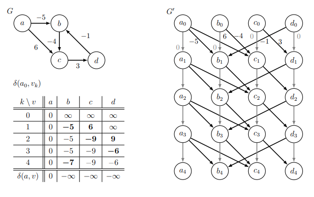
INF = float('inf')

def bellman_ford(adj, w, s):
    # initialization
	d = [INF for _ in adj]     
    parent = [None for _ in adj]
    d[s], parent[s] = 0, s
    V = len(adj)
    
    # construct shortest paths in rounds
    for k in range(V-1):
        for u in range(V):
            for v in adj[u]:
                try_to_relax(adj, w, d, parent, u, v)
	
    # check for negative weight cycles accessible from s
    for u in range(V):
        for v in adj[u]:
            if d[v] > d[u] + w(u, v):
            	raise Exception("found a negative weight in cycle!")
	return d, parent

TBC

Running Time

$G’$ has size $O( V ( V + \vert E \vert ))$ and can be constructed in as much time
Running DAG Relaxation on $G’$takes linear time in the size of $G’$
Does $O(1)$ work for each vertex reachable from a witness
Finding reachability of a witness takes $O(\vert E \vert )$ time, with at most $O(\vert V \vert )$ witnesses: $O(\vert V \vert \vert E \vert )$
(Alternatively, connect super node $x$ to witnesses via 0-weight edges, linear search from $x$)
Pruning $G$ at start to only subgraph reachable from $s$ yields $O(\vert V \vert \vert E \vert )$ time algorithm

13 Dijkstra’s Algorithm

Notes

Non-negative Edge Weights

Idea! Generalize BFS approach to weighted graphs:
- Grow a sphere centered at source s
- Repeatedly explore closer vertices before further ones
- But how to explore closer vertices if you don’t know distances beforehand? :(
Observation 1: If weights non-negative, monotonic distance increasing along shortest paths
- i.e., if vertex $u$ appears on a shortest path from $s$ to $v$, then $\delta(s, u) \leq \delta(s, v)$
- Let $V_x \subset V$ be the subset of vertices reachable within distance $\leq x$ from $s$
- If $v \in V_x$ then any shortest path from $s$ to $v$ only contains vertices from $V_x$
- Perhaps grow $V_x$ one vertex at a time! (but growing for every $x$ is slow if weights large)
Observation 2: Can solve SSSP fast if given order of vertices in increasing distance from $s$
- Remove edges that go against this order (since cannot participate in shortest paths)
- May still have cycles if zero-weight edges: repeatedly collapse into single vertices
- Compute $\delta(s, v)$ for each $v\in V$ using DAG relaxation in $O(\vert V \vert + \vert E \vert )$ time

Dijkstra’s Algorithm

Idea! Relax edges from each vertex in increasing order of distance from source $s$
Idea! Efficiently find next vertex in the order using a data structure

Changeable Priority Queue $Q$ on items with keys and unique IDs, supporting operations:

Operation	Specification
`Q.build(X)`	initialize $Q$ with items in iterator `X`
`Q.delete_min()`	remove an item with minimum key
`Q.decrease_key(id, k)`	find stored item with ID `id` and change key to `k`

Implement by cross-linking a Priority Queue $Q’$ and a Dictionary $D$ mapping IDs into $Q’$
Assume vertex IDs are integers from $0$ to $\vert V \vert -1$ so can use a direct access array for D
For brevity, say item x is the tuple $(x.id, x.key)$
Set $d(s, v) = \infty$ for all $v \in V$, then set $d(s,s) = 0$
Build changeable priority queue $Q$ with an item $(v, d(s, v))$ for each vertex $v \in V$
- For vertex $v$ in outgoing adjacencies $Adj^+(u)$:
  - If $d(s, v)>d(s,u) + w(u, v)$:
    - Relax edge $(u, v)$, i.e., set $d(s, v) = d(s, u) + w(u, v)$
    - Decrease the key of $v$ in $Q$ to new estimate $d(s, v)$

dijkstra

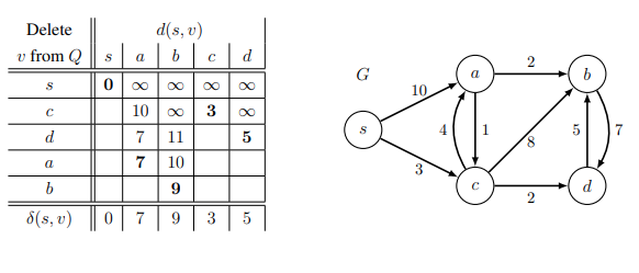
def dijkstra(adj, w, s):
    d = [INF for _ in adj]
    parent = [None for _ in adj]
    d[s], parent[s] = 0, s
    Q = PriorityQueue()    
    V = len(adj)
    for v in range(V):
        Q.insert(v, d[v])   # label and key
    for _ in range(V):
        u = Q.extract_min() # get label for item with min key
       	for v in adj[u]:
            try_to_relax(adj, w, d, parent, u, v)
            Q.decrease_key(v, d[v]) # alter key for given label
	return d, parent


class PriorityQueue:
    def __init__(self):
        self.A = {}
        
    def insert(self, label, key):
        self.A[label] = key
    
    def extract_min(self):
        min_label = None
        for label in self.A:
            if (min_label is None) or (self.A[label] < self.A[min_label]):
                min_label = label
        del self.A[min_label]
        return min_label
    
    def decrease_key(self, label, key):
        if (label in self.A) and (key < self.A[label]):
            self.A[label] = key
            
            
class Item:
    def __init__(self, label, key):
        self.label, self.key = label, key
    
    def __lt__(self, other):
        return self.key < other.key
        
class PriorityQueue:
    def __init__(self):
        self.A = []
        self.label_2_idx = dict()
        
    def insert(self, label, key):
        item = Item(label, key)
        self.A.append(item)
        idx= len(self.A) - 1
        self.label_2_idx[label] = idx
        heapq._siftdown(self.A, 0, idx)
        
    def extract_min(self):
        label = self.A[0].label
        self.A[0], self.A[-1] = self.A[-1], self.A[0]
        self.label_2_idx[self.A[0].label] = 0
        self.label_2_idx.pop(self.A[-1].label)
        self.A.pop()
        if self.A: heapq._siftup(self.A, 0)
        return label
    
    def decrease_key(self, label, key):
        if label in self.label_2_idx:
            idx = self.label_2_idx[label]
            if self.A[idx].key < key:
                self.A[idx].key = key
                heapq._siftdown(self.A, 0, idx)

Correctness

Claim: At end of Dijkstra’s algorithm $d(s, v) = \delta(s, v)$ for all $v \in V$
Proof:
- If relaxation sets $d(s, v)$ to $\delta(s, v)$, then $d(s, v) = \delta(s, v)$ at the end of the algorithm
 - Relaxation can only decrease estimates $d(s, v)$
 - Relaxation is safe, i.e., maintains that each $d(s, v)$ is weight of a path to $v$ (or $\infty$)
- Suffices to show $d(s, v) = \delta(s, v)$ when vertex $v$ is removed from $Q$
 - Proof by induction on first $k$ vertices removed from $Q$
 - Base Case ($k$ = 1): $s$ is first vertex removed from $Q$, and $d(s, s) = 0 = δ(s, s)$
 - Inductive Step: Assume true for $k < k’$ , consider $k’$ th vertex $v_0$ removed from $Q$
 - Consider some shortest path $π$ from $s$ to $v’$, with $w(π) = δ(s, v’ )$
 - Let $(x, y)$ be the first edge in $π$ where $y$ is not among first $k’ - 1$ (perhaps $y = v’$ )
 - When $x$ was removed from $Q$, $d(s, x) = δ(s, x)$ by induction, so: $\begin{align} d(s, y) &\leq \delta(s, x) + w(x, y) \\ &=\delta(s, y) \\ &\leq \delta(s, v') \\ &\leq d(s, v') \\ &\leq d(s, y) \\ \end{align}$
 - So $d(s, v’) = \delta(s, v’)$ as desired

Running Time

Count operations on changeable priority queue Q, assuming it contains n items:

Operation	Time	Occurrences in Dijkstra
`Q.build(X)`	$B_n$	1
`Q.delete_min()`	$M_n$	\|V\|
`Q.decrease_key(id, k)`	$D_n$	\|E\|

Total running time is $O(B_{\vert V \vert } + \vert V \vert \cdot M_{\vert V \vert } + \vert E \vert \cdot D_{\vert V \vert })$
Assume pruned graph to search only vertices reachable from the source, so $ V = O(\vert E \vert )$

TBC

15 Recursive Algorithms

Notes

Design your own recursive algorith

Constant-sized program to solve arbitrary input
Need looping or recursion, analyze by induction
Recursive function call: vertex in a graph, directed edge from $A\rightarrow B$ if $B$ calls $A$
Dependency graph of recursive calls must be acyclic (if can terminate)
Classify based on shape of graph

Class	Graph
Brute Force	Star
Decrease & Conquer	Chain
Divide & Conquer	Tree
Dynamic Programming	DAG
Greedy / Incremental	Subgraph

Hard part is thinking inductively to construct recurrence on subproblems
How to solve a problem recursively (SRT BOT)
- Subproblem definition
- Relate subproblem solutions recursively
- Topological order on subproblems ($\Rightarrow$ subproblem DAG)
- Base cases of relation
- Original problem solution via subproblems(s)
- Time analysis

Merge Sort in SRT BOT Framework

Merge sorting an array $A$ of $n$ elements can be expressed in SRT BOT as follows:
Subproblems: $S(i,j)=$ sorted array on elements of $A[i:j]$ for $i \leq i \leq j \leq n$
Relation: $S(i,j) = merge(S(i, m), S(m, j))$ where $m=\lfloor (i+j) / 2 \rfloor$
Topological order: Increasing $j - i$
Base cases: $S(i, i + 1) = [A[i]]$
Original: $S(0, n)$
Time: $T(n) = 2T(n/2) + O(n) = O(nlogn)$

Fibonacci Numbers

Compute the $n$th Fibonacci number $F_n$
Subproblems: $F(i)=$ the $i$th Fibonacci number $F_i$ for $i \in {0,1,…, n}$
Relation: $F(i) = F(i-1)+F(i-2)$ (definition of Fibonacci numbers)
Topological order: Increasing $i$
Base cases: $F(0) = 0, F(1) = 1$
Original problem: $F(n)$

def fib(n):
    if n < 2: return n
    return fib(n-1) + fib(n-2)

Divide and conquer implies a tree of recursive calls
Time: $T(n) = T(n-1)+T(n-2) + O(1) > 2T(n-2), T(n) = \Omega(2 ^{n/2})$ exponential… :(
Subproblem $F(k)$ computed more than once! ($F(n-k)$ times)
Can we avoid this waste?

Re-using Subproblem Solutions

Either:
- Top down: record subproblem solutions in a memo and re-use
- Bottom up: solve subproblems in topological sort order (usually via loops)
For Fibonacci, $n + 1$ subproblems (vertices) and $<2n$ dependencies (edges)
Time to compute is then $O(n)$ additions

def fib(n):
    memo = dict()
    def F(i):
        if i < 2: return i
       	if i not in memo:
            memo[i] = F(i-1) + F(i-2)
        return memo[i]
   return F(n)

def fib(n):
    F = dict()
    F[0], F[1] = 0, 1
    for i in range(2, n+1):
        F[i] = F[i-1] + F[i-2]
    return F[n]

A subtlety is that Fibonacci numbers grow to $\Theta(n)$ bits long, potentially $\gg$ word size $w$
Each addition costs $O(\lceil n / w \rceil)$ time
So total cost is $O(n\lceil n / w \rceil) = O(n + n^2/w)$ time

Dynamic Programming

Weird name coined by Richard Bellman
- Wanted government funding, needed cool name to disguise doing mathematics!
- Updating (dynamic) a plan or schedule (program)
Existence of recursive solution implies decomposable subproblems
Recursive algorithm implies a graph of computation
Dynamic programming if subproblem dependencies overlap (DAG, in-degree > 1)
“Recurse but re-use” (Top down: record and lookup subproblem solutions)
“Careful brute force” (Bottom up: do each subproblem in order)
Often useful for counting/optimization problems: almost trivially correct recurrences

How to Solve a Problem Recursively (SRT BOT)

Subproblem definition subproblem $x\in X$
- Describe the meaning of a subproblem in words, in terms of parameters
- Often subsets of input: prefixes, suffixes, contiguous substrings of a sequence
- Often record partial state: add subproblems by incrementing some auxiliary variable
Relate subproblem solutions recursively $x(i) = f(x(j),…)$ for one or more $j < i$
Topological order: to argue relation is acyclic and subproblems form a DAG
Base cases
- State solutions for all (reachable) independent subproblems where relation breaks down
Original problem
- Show how to compute solution to original problem from solutions to subproblem(s)
- Possibly use parent pointers to recover actual solution, not just objective function
Time analysis
- $\Sigma_{x\in X}work(x), $ or if $work(x)=O(W)$ for all $x\in X$, then $ X \cdot O(W)$
- $work(x)$ measures non-recursive work in relation; treat recursions as taking $O(1)$ time

DAG Shortest Paths

DAG SSSP problem: given a DAG G and vertex $s$, compute $\delta(s, v)$ for all $v\in V$
Subproblems: $\delta(s, v)$ for all $v\in V$
Relation: $\delta(s, v)=min{\delta(s, u) + w(u, v) \vert u \in Adj^-(v)} \cup {\infty}$
Topological order: Topological order of G
Base case: $\delta(s, s) = 0$
Original: All subproblem
Time: $\Sigma_{v\in V}O(1+\vert A dj^-(v)\vert ) = O(\vert V \vert +\vert E \vert )$
DAG Relaxation computes the same min values as this dynamic program, just
- step-by-step (if new value < min, update min via edge relaxation), and
- from the perspective of $u$ and $Adj^+(u)$ instead of $v$ and $Adj^-(v)$

How to Relate Subproblem Solutions

The general approach we’re following to define a relation on subproblem solutions:
- Identify a question about a subproblem solution that, if you knew the answer to, would reduce to “smaller” subproblem(s)
- Then locally brute-force the question by trying all possible answers, and taking the best
- Alternatively, we can think of correctly guessing the answer to the question, and directly recursing; but then we actually check all possible guesses, and return the “best”
The key for efficiency is for the question to have a small (polynomial) number of possible answers, so brute forcing is not too expensive
Often (but not always) the non-recursive work to compute the relation is equal to the number of answers we’re trying

16 Dynamic Programming Subproblems

Notes

Longest Common Subsequence (LCS)

Given two strings $A$ and $B$, find a longest (not necessarily contiguous) subsequence of $A$ that is also a subsequence of $B$.
Example: $A=hieroglyphology \ B=michaelangelo$
Solution: $hello$ or $heglo$ or $iello$ or $ieglo$, all length 5
Maximization problem on length of subsequence

Subproblems:
- $x(i, j)=$ length of the longest common subsequence of suffixes $A[i:]$ and $B[j:]$
- For $0\leq i \leq \vert A \vert $ and $0 \leq j \leq \vert B \vert $
Relate:
- Either first characters match or they don’t
- If first characters match, some longest common subsequence will use them
- (if no LCS uses first matched pair, using it will only improve solution)
- (if an LCS uses first in $A[i]$ but not first in $B[j]$, matching $B[j]$ is also optimal)
- If they do not match, they cannot both be in a longest common subsequence
- Guess whether $A[i]$ or $B[j]$ is not in LCS
- $x(i, j) = \begin{cases} x(i + 1, j+1) + 1 \qquad if A[i] = B[j]\max{x(i+1, j), x(i,j+1)} \qquad otherwise \end{cases}$
Topological order:
- Subproblem $x(i, j)$ depend only on strictly larger $i$ or $j$ or both
- Simplest order to state: Decreasing $i + j$
- Nice order for bottom-up code: Decreasing $i$, then decreasing $j$
Base
- $x(i, \vert B \vert ) = x(\vert A \vert , j)=0$ (one string is empty)
Original problem
- Length of longest common subsequence of $A$ and $B$ is $x(0,0)$
- Store parent pointers to reconstruct subsequencce
- If the parent pointer increases both indices, add that character to LCS
Time:
- # subproblems: $(\vert A \vert + 1)\cdot(\vert B \vert + 1)$
- work per subproblem: $O(1)$
- $O(\vert A \vert \ cdot \vert B \vert ) $ running time

def lcs(A, B):
    a, b = len(A), len(B)
    x = [[0] * (b + 1) for _ in range(a + 1)]
    for i in reversed(range(a)):
        for j in reversed(range(b)):
            if A[i] == B[j]:
                x[i][j] = x[i + 1][j + 1] + 1
            else:
                x[i][j] = max(x[i + 1][j], x[i][j + 1])
	return x[0][0]

def lcs(A, B):
    a, b = len(A), len(B)
    x = [[0] * (b + 1) for _ in range(a + 1)]
    for i in range(1, a + 1):
        for j in range(1, b + 1):
            if A[i] == B[j]:
                x[i][j] = x[i - 1][j - 1] + 1
            else:
                x[i][j] = max(x[i - 1][j], x[i][j - 1])
	return x[0][0]

Longest Increasing Subsequence (LIS)

Given a string $A$, find a longest (not necessarily contiguous) subsequence of $A$ that strictly increases (lexicographically).
Example: $A= carbohydrate$
Solution: $abort$ of length 5
Maximization problem on length of subsequence
Attempted solution:
- Natural subproblems are prefixes or suffixes of $A$, say suffix $A[i :]$
- Natural question about LIS of $A[i :]$: is $A[i]$ in the LIS? (2 possible answers)
- But then how do we recurse on $A[i + 1 :]$ and guarantee increasing subsequence?
- Fix: add constraint to subproblems to give enough structure to achieve increasing property

Subproblems
- $x(i)$ = length of longest increasing subsequence of suffix $A[i:]$ that includes $A[i]$
- For $0\leq i \leq \vert A \vert$
Relate
- We’re told that $A[i]$ is in LIS (first element)
- Next question: what is the second element of LIS?
 - Could be any $A[j]$ where $j > i$ and $A[j] > A[i]$ (so increasing)
 - Or $A[i]$ might be the last element of LIS
- \[x(i) = max\{1 + x(j) \vert i < j < \vert A \vert , A[j] > A[i]\} \cup \{1\}\]
Topological order:
- Decreasing $i$
Base
- No base case necessary, because we consider the possibility that $A[i]$ is last
Original problem
- What is the first element of LIS? Guess!
- Length of LIS of $A$ is $max\{x(i) \vert 0\leq i < \vert A \vert \}$
- Store parent pointers to reconstruct subsequence
Time
- # subproblems: $\vert A \vert$
- work per subproblem $O( \vert A \vert )$
- $O( \vert A \vert ^2)$ running time
- speed up to $O( \vert A \vert log \vert A \vert )$ by doing only $O(log \vert A \vert )$ work per subproblem, via AVL tree augmentation

def lis(A):
    a = len(A)
    x = [1] * a
    for i in reversed(range(a)):
        for j in range(i, a):
            if A[j] > A[i]:
                x[i] = max(x[i], 1 + x[j])
	return max(x)

Alternating Coin Game

Given sequence of n coins of value $v_0, v_1,...,v_{n1}$
Two players (“me” and “you”) take turns
In a turn, take first or last coin among remaining coins
My goal is to maximize total value of my taken coins, where I go first
First solution exploits that this is a zero-sum game: I take all coins you don’t

Subproblems
- Choose subproblems that correspond to the state of the game
- For every contiguous subsequence of coins from $i$ to $j$, $0\leq i \leq j < n$
- $x(i, j)=$ maximum total value I can take starting from coins of values $v_i, ..., v_j$
Relate
- I must choose either coin $i$ or coin $j$ (Guess!)
- Then it’s your turn, so you’ll get values $x(i+1, j)$ or $x(i, j-1)$ respectively
- To figure out how much value I get, subtract this from total coin values
- $x(i,j) = max\{v_i + \Sigma_{k=i+1}^{j} v_k \qquad x(i + 1, j), v_j + \Sigma_{k=i}^{j}v_k \qquad x(i, j-1)\}$ ???
Topological order
- Increasing $j - i$
Base
- \[x(i,i) = v_i\]
Original problem
- \[x(0, n- 1)\]
- store parent pointers to reconstruct strategy
Time
- # subproblems: $\Theta(n^2)$
- work per subproblem: $\Theta(n)$ to compute sums
- $\Theta(n^3)$ running time
- Speed up to $\Theta(n^2)$ time by pre-computing all sums $\Sigma_{k=i}^{j}v_k$ in $\Theta(n^2)$ time via dynamic programming

Second solution uses subproblem expansion: add subproblems for when you move next

Subproblems
- Choose subproblems that correspond to the full state of the game
- Contiguous subsequence of coins from $i$ to $j$, and which player $p$ goes next
- $x(i, j, p) =$ maximum total value I can take when player $p \in \{me, you\}$ starts from coins of values $v_i,...,v_j$
Relate
- Player $p$ must choose either coin $i$ or coin $j$ (Guess!)
- If $p =$ me, then I get the value; otherwise, I get nothing
- Then it’s the other player’s turn
- \[x(i, j, me) = max\{v_i + x(i + 1, j, you), v_j + x(i, j - 1, you)\}\]
- \[x(i, j, you) = min\{x(i + 1, j, me), x(i, j-1, me)\}\]
Topological order
- Increasing $j - i$
Base
- \[x(i, i, me) = v_i\]
- \[x(i,i,you)=0\]
Original problem
- \[x(0, n-1, me)\]
- Store parent pointers to reconstruct strategy
Time
- # subproblems: $\Theta(n^2)$
- work per subproblem: $\Theta(1)$
- $\Theta(n^2)$ running time

Yet another alternative solution.

def coin_game(coins):
    n = len(coins)
    dp = [[0] * n for _ in range(n)]    
    for i in reversed(range(n)):
        for j in range(i, n):
            if i == j: 
                d[i][j] = coins[i]
            else:
                dp[i][j] = max(coins[i] - dp[i+1][j], coins[j] - dp[i][j-1])
	return dp[0][n-1] >= 0

def coin_game(coins):
    n = len(coins)
    dp = [[0] * n for _ in range(n)]
    parents = dict()
    
    for i in reversed(range(n)):
        for j in range(i, n):
            if i == j: 
                d[i][j] = coins[i]
                parents[(l, r)] = ((l, r), coins[l])
            else:
                a = coins[i] - dp[i+1][j]
                b = coins[j] - dp[i][j-1]
                if a > b:
                    dp[i][j] = a
                    parents[(l, r)] = ((l+1, r), nums[l])
                else:
                    dp[i][j] = b
                    parents[(l, r)] = ((l, r-1), nums[r])
                    
	if dp[0][n-1] >= 0
		state = (0, n-1)
        turn = 1
        while parents[state][0] != state:
            print(f"player {turn % 2} took {parents[state][1]}")
            state = parents[state][0]
            turn += 1
        
	return dp[0][n-1] >= 0

Subproblem Constraints and Expansion

We’ve now seen two examples of constraining or expanding subproblems
If you find yourself lacking information to check the desired conditions of the problem, or lack the natural subproblem to recurse on, try subproblem constraint/expansion!
More subproblems and constraints give the relation more to work with, so can make DP more feasible
Usually a trade-off between number of subproblems and branching/complexity of relation

17 Dynamic Programming III

Notes

Single-Source Shortest Paths Revisited

Subproblems
- Expand subproblems to add information to make acyclic!
- $\delta_k(s,v)=$ weight of shortest path from $s$ to $v$ using at most $k$ edges
- For $v\in V$ and $0 \leq k \leq \vert V \vert$
Relate:
- Guess last edge $(u, v)$ on shortest path from $s$ to $v$
- \[\delta_k(s, v) = min\{\delta_{k-1}(s, u) + w(u, v) \vert (u, v) \in E\}\ \cup\ \{\delta_{k-1}(s, v)\}\]
Topological order:
- Increasing k: subproblems depend on subproblems only with strictly smaller $k$.
base
- $\delta_{0}(s, s)=0$ and $\delta_0(s, v) = \infty$ for $v \neq s$ (no edges)
Original problem
- If has finte shortest path, then $\delta(s, v) = \delta_{\vert V \vert- 1}(s, v)$
- Otherwise some $\delta_{\vert V \vert }(s, v) < \delta_{\vert V \vert - 1}(s, v)$, so path contains a negative-weight cycle
- Can keep track of parent pointers to subproblem that minimized recurrence
Time
- # subproblems: $\vert V \vert \times (\vert V \vert +1)$
- Work for subproblem $\delta_k(s,v): O(deg_{in}(v))$ $\Sigma_{k=0}^{\vert V \vert } \Sigma_{v\in V}O(deg_{in}(v)) = \Sigma_{k=0}^{\vert V \vert } O(\vert E \vert ) =O(\vert V \vert \ cdot\vert E \vert )$

This is just Bellman-Ford! (computed in a slightly different order)

All-Pairs Shortest Paths: Floyd-Warshall

Could define subproblem $\delta_k(u, v)=$ minimum weight of path from $u$ to $v$ using at most $k$ edges, as in Bellman-Ford
Resulting running time is $\vert V \vert$ times Bellman-Ford, i.e., $O(\vert V \vert ^2 \cdot \vert E \vert ) = O(\vert V \vert ^4)$
Know a better algorithm from L14: Johnson achieves $O(\vert V \vert ^2log \vert V+\vert V \vert \cdot\vert E \vert )=O(\vert V \vert ^3)$
Can achieve $\Theta(\vert V \vert ^3)$ running time (matching Johnson for dense graphs) with a simple dynamic program, called Floyd-Warshall.
Number vertices so that $V=\{1,...,\vert V \vert \}$

Subproblems:
- $d(u, v, k)=$ minimum weight of a path from $u$ to $v$ that only uses vertices from $\{1,2,...,k\} \cup \{u, v\}$
- For $u, v \in V$ and $1\leq k \leq \vert V \vert$
Relate
- \[x(u, v, k)= min\{x(u, k, k-1) + x(k,v,k-1), x(u, v, k-1)\}\]
- Only constant branching! No longer guessing previous vertex/edge
Topological order
- Increasing $k$: relation depends only on smaller $k$
Base
- \[x(u, u, 0) = 0\]
- $x(u, v, 0) = w(u, v)$ if $(u, v)\in E$
- $x(u,v,0)=\infty$ if none of the above
Original problem
- $x(u, v, \vert V \vert )$ for all $u, v \in V$
Time
- $O(\vert V \vert ^3)$ subproblems
- Each $O(1)$ work
- $O(\vert V \vert ^3)$ in total
- Constant number of dependencies per subproblem brings the factor of $O(\vert E \vert)$ in the running time down to $O(\vert V \vert)$

input	constant	logarithmic	linear	log-linear	quadratic	polynomial	exponential
\(n\)	\(Θ(1)\)	\(Θ(log n)\)	\(Θ(n)\)	\(Θ(n log n)\)	\(Θ(n^2)\)	\(Θ(n^c )\)	\(2^Θ(n^c)\)
\(1000\)	\(1\)	\(≈ 10\)	\(1000\)	\(≈ 10,000\)	\(1,000,000\)	\(1000^c\)	\(2^1000 ≈ 10^301\)
Time	\(1 ns\)	\(10 ns\)	\(1 µs\)	\(10 µs\)	\(1 ms\)	\(10^{(3c-9)} s\)	\(10^281 millenia\)

Sequence Data Structure	API Type			Worst Case \(O(\cdot)\)
Array	Container	Static	Dynamic
API	`build(x)`	`get_at(i)` `set_at(i)`	`insert_first(x)` `delete_first()`	`insert_last(x)` `delete_last()`	`insert_at(i, x)` `delete_at(i)`
Static Array	\(n\)	\(1\)	\(n\)	\(n\)	\(n\)
Linked List	\(n\)	\(n\)	\(1\)	\(n\) # 1 if we keep track of tail	\(n\)
Dynamic Array	\(n\)	\(1\)	\(n\)	\(1_{(a)}\)	\(n\)

case	solution	conditions
1	\(T(n) = \Theta(n^{log_b^a})\)	\(f(n) = \Theta(n^{log_b^{a-\epsilon}})\) for some constant \(ε > 0\)
2	\(T(n) = \Theta(n^{log_b^a}log^{k+1}n)\)	\(T(n) = \Theta(n^{log_b^a}log^{k}n)\) for some constant \(k ≥ 0\)
3	\(T(n) = \Theta(f(n))\)	\(f(n) = \Theta(n^{log_b^{a+\epsilon}})\) for some constant \(ε > 0\) and \(af(n/b) < cf(n)\) for some constant \(0 < c < 1\)

Data Structure	API Type			Worst Case \(O(\cdot)\)
Set	Container	Static	Dynamic
API	`build(x)`	`find(k)`	`insert(k)` `delete(k)`	`find_min()` `find_max()`	`find_prev(k)` `find_next(k)`
Array	\(n\)	\(n\)	\(n\)	\(n\)	\(n\)
Sorted Array	\(nlogn\)	\(logn\)	\(n\)	\(1\)	\(logn\)
Direct Access Array	\(u\)	\(1\)	\(1\)	\(u\)	\(u\)
Hash Table	\(n_{(e)}\)	\(1_{e}\)	\(1_{(a)(e)}\)	\(n\)	\(n\)

Sequence Data Structure	API Type			Worst Case $O(\cdot)$
Array	Container	Static	Dynamic
API	`build(x)`	`get_at(i)` `set_at(i)`	`insert_first(x)` `delete_first()`	`insert_last(x)` `delete_last()`	`insert_at(i, x)` `delete_at(i)`
Static Array	\(n\)	\(1\)	\(n\)	\(n\)	\(n\)
Linked List	\(n\)	\(n\)	\(1\)	\(n\) # 1 if we keep track of tail	\(n\)
Dynamic Array	\(n\)	\(1\)	\(n\)	$1_{(a)}$	\(n\)
Goal	\(n\)	\(logn\)	\(logn\)	\(logn\)	\(logn\)

case	solution	conditions	intuition
1	\(T(n) = \Theta(n^{log_b^a})\)	\(c < log_b^a\)	Work done at leaves dominates
2	\(T(n) = \Theta(n^{c}log^{n})\)	\(c=log_b^a\)	Work balanced across the tree
3	\(T(n) = \Theta(n^c)\)	\(c>log_b^a\)	Work done at root dominates

1 Introduction

Notes

More on Asymptotic Notation

2 Data Structures

Notes

Data Structure Interfaces

Sequence Interface (L02, L07)

Set Interface (L03-L08)

Array Sequence

Linked List Sequence

Dynamic Array Sequence

Amortized Analysis

Dynamic Array Deletion

3 Sorting

Notes

Set Interface

Sorting

Permutation Sort

Solving Recurrences

Selection Sort

Insertion Sort

Merge Sort

Master Theorem

4 Hashing

Notes

Comparison Model

Decision Tree

Comparison Search Lower Bound

Direct Access Array

Hashing

Chaining

Hash Functions

Division (bad): \(h(k) = k \ \mod \ m\)

Universal (good, theoretically): \(h_{ab}{(k)}=(((ak+b) \mod \ p) \mod \ m)\)

Dynamic

5 Linear Sorting

Notes

Comparison Sort Lower Bound

Direct Access Array Sort

Tuple Sort

Counting Sort

Radix Sort

6 Binary Trees, Part 1

Notes

How? Binary Trees!

Terminology

Tree Navigation

Dynamic Operations

Application: Set

Application: Sequence

7 Binary Tree II: AVL

Notes

Height Balance

Rotations

Rotations Suffice

AVL Trees: Height Balance

Computing Height

Steps to Augment a Binary Tree

Application: Sequence

Conclusion

Application: Sorting

8 Binary Heaps

Notes

Priority Queue Interface

Priority Queue Sort

Priority Queue: Set AVL Tree

Priority Queue: Array

Priority Queue: Sorted Array

Array as a Complete Binary Tree

Implicit Complete Tree

Binary Heaps

Heap Insert

Heap Delete Max

Heap Sort

In-place Priority Queue Sort

Linear Build Heap

Sequence AVL Tree Priority Queue

Set vs. Multiset

9 Breadth-First Search

Notes