Storage and Retrieval

Database

On the most fundamental level, a database needs to do two things: when you give it some data, it should store the data, and when you ask it again later, it should give the data back to you.

• Log: append only data file.

• Index: additional data structure to speed up search.

• In order to efficiently find the value for a particular key in the database, we need index.
• For writes, it’s hard to beat the performance of simply appending to a file, because that’s the simplest possible write operation. Any kind of index usually slows down writes, because the index also needs to be updated every time data is written.

This is an important trade-off in storage systems: well-chosen indexes speed up read queries, but every index slows down writes.

Hash Indexes

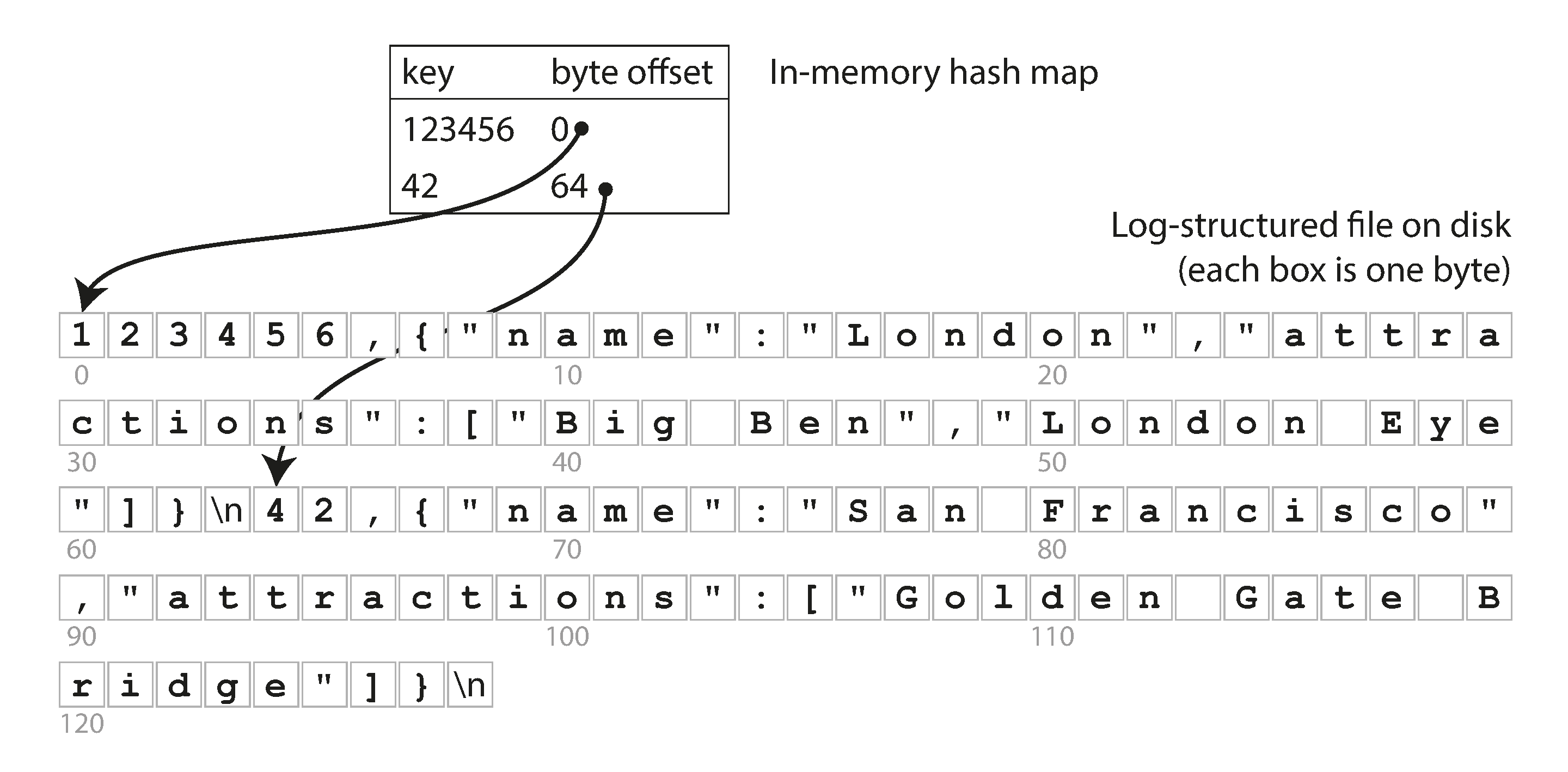
• the simplest possible indexing strategy is this: keep an in-memory hash map where every key is mapped to a byte offset in the data file

Compaction

To avoid running out of disk, a good solution is to break the log into segments of a certain size by closing a segment file when it reaches a certain size, and making subsequent writes to a new segment file. We can then perform compaction on these segments.

Compaction means throwing away duplicate keys in the log, and keeping only the most recent update for each key. We can also merge several segments together at the same time as performing the compaction.

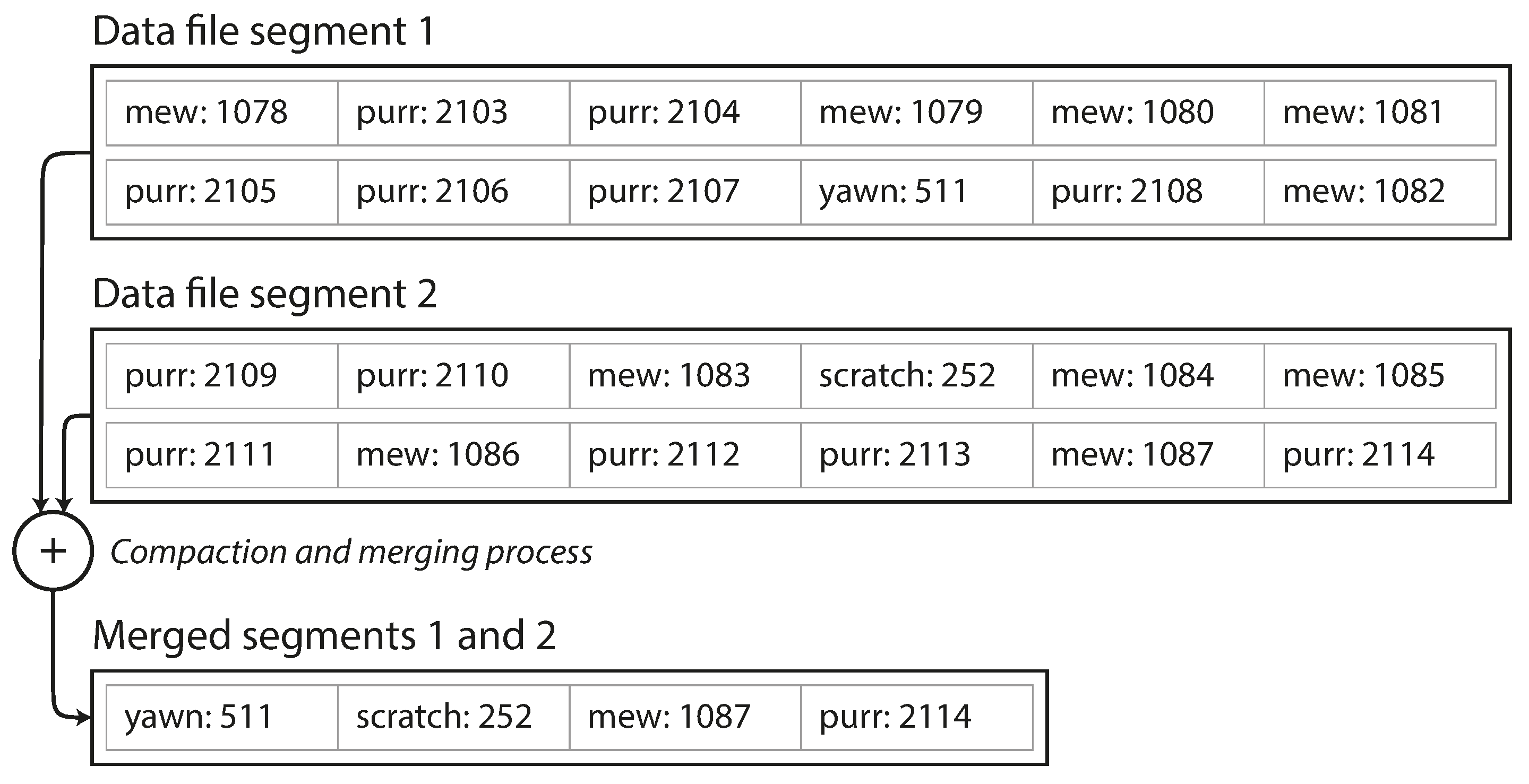
The merging and compaction of frozen segments can be done in a background thread, and while it is going on, we can still continue to serve read and write requests as normal, using the old segment files. After the merging process is complete, we switch read requests to using the new merged segment instead of the old segments—and then the old segment files can simply be deleted.

Each segment now has its own in-memory hash table, mapping keys to file offsets. In order to find the value for a key, we first check the most recent segment’s hash map; if the key is not present we check the second-most-recent segment, and so on.

Implementation details

1. File format
   • use a binary format that first encodes the length of a string in bytes, followed by the raw string.
2. Deleting records
   • append a special deletion record to the data file (sometimes called a tombstone).
3. Crash recovery
   • storing a snapshot of each segment’s hash map on disk, which can be loaded into memory more quickly.
4. Partially written records
   • use checksums, allowing corrupted parts of the log to be detected and ignored.
5. Concurrency control
   • only one writer thread. Data file segments are append-only and otherwise immutable, so they can be read concurrently by multiple threads.

SSTables and LSM-Trees

Sorted String Table, or SSTable

• we require that the sequence of key-value pairs is sorted by key
• We also require that each key only appears once within each merged segment file (the compaction process already ensures that)

Pros:

• merging segments is simple and efficient, even if the files are bigger than the available memory. The approach is like the one used in the mergesort.
• you still need an in-memory index to tell you the offsets for some of the keys, but it can be sparse.
• it is possible to group ranges of records into a block and compress it before writing it to disk.

Constructing and maintaining SSTables

• Use an in memory balanced search tree data structure like red-black tree or AVL tree.
• When a write comes in, add it to an in-memory balanced tree data structure (sometimes called memtable).
• When the memtable gets bigger than some threshold—typically a few megabytes—write it out to disk as an SSTable file. This can be done efficiently because the tree already maintains the key-value pairs sorted by key. The new SSTable file becomes the most recent segment of the database. While the SSTable is being written out to disk, writes can continue to a new memtable instance.
• In order to serve a read request, first try to find the key in the memtable, then in the most recent on-disk segment, then in the next-older segment, etc.
• From time to time, run a merging and compaction process in the background to combine segment files and to discard overwritten or deleted values.
• we can keep a separate log on disk to which every write is immediately appended, just like in the previous section. That log is not in sorted order, but that doesn’t matter, because its only purpose is to restore the memtable after a crash.

LevelDB and RocksDB are pretty much using this scheme, Similar storage engines are used in Cassandra and HBase [8], both of which were inspired by Google’s Bigtable paper [9] (which introduced the terms SSTable and memtable)

Log-Structured Merge-Tree (or LSM-Tree)

Lucene, an indexing engine for full-text search used by Elasticsearch and Solr, uses a similar method for storing its term dictionary.

the LSM-tree algorithm can be slow when looking up keys that do not exist in the database: you have to check the memtable, then the segments all the way back to the oldest (possibly having to read from disk for each one) before you can be sure that the key does not exist. In order to optimize this kind of access, storage engines often use additional Bloom filters [15]. (A Bloom filter is a memory-efficient data structure for approximating the contents of a set. It can tell you if a key does not appear in the database, and thus saves many unnecessary disk reads for nonexistent keys.

There are also different strategies to determine the order and timing of how SSTables are compacted and merged. The most common options are size-tiered and leveled compaction.

• In size-tiered compaction, newer and smaller SSTables are successively merged into older and larger SSTables.
• In leveled compaction, the key range is split up into smaller SSTables and older data is moved into separate “levels,” which allows the compaction to proceed more incrementally and use less disk space.

B-Trees

They remain the standard index implementation in almost all relational databases, and many nonrelational databases use them too.

• B-trees keep key-value pairs sorted by key, which allows efficient keyvalue lookups and range queries.
• B-trees break the database down into fixed-size blocks or pages, traditionally 4 KB in size (sometimes bigger), and read or write one page at a time.
• Each page can be identified using an address or location, which allows one page to refer to another—similar to a pointer, but on disk instead of in memory. We can use these page references to construct a tree of pages.

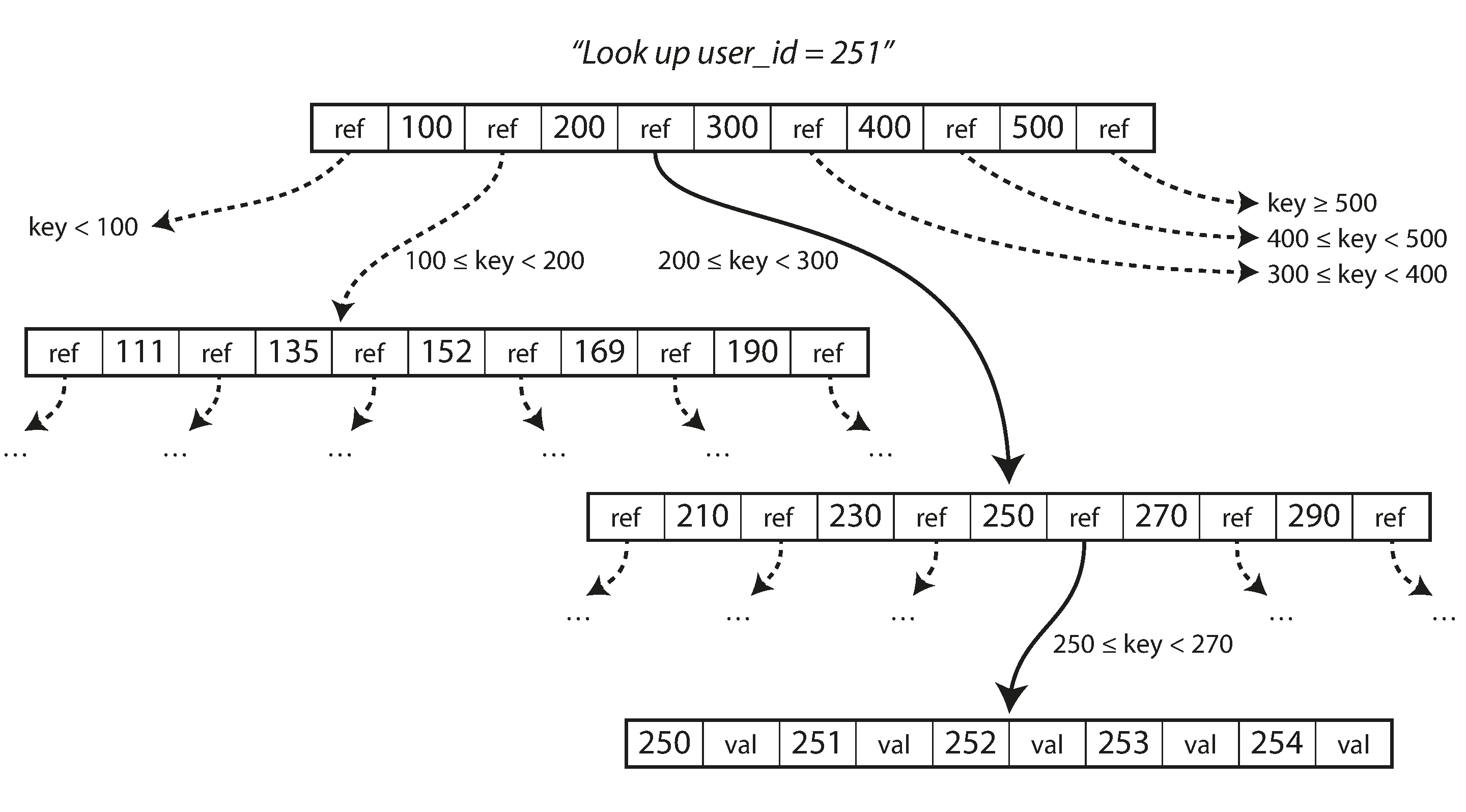
This algorithm ensures that the tree remains balanced: a B-tree with n keys always has a depth of O(log n). Most databases can fit into a B-tree that is three or four levels deep, so you don’t need to follow many page references to find the page you are looking for. (A four-level tree of 4 KB pages with a branching factor of 500 can store up to 256 TB.)

In order to make the database resilient to crashes, it is common for B-tree implementations to include an additional data structure on disk: a write-ahead log (WAL, also known as a redo log). This is an append-only file to which every B-tree modification must be written before it can be applied to the pages of the tree itself. When the database comes back up after a crash, this log is used to restore the B-tree back to a consistent state [5, 20].

Comparing B-Trees and LSM-Trees

• LSM-trees are typically faster for writes, whereas B-trees are thought to be faster for reads.
• Reads are typically slower on LSM-trees because they have to check several different data structures and SSTables at different stages of compaction.

In Memory Databases

As RAM becomes cheaper, the cost-per-gigabyte argument is eroded. Many datasets are simply not that big, so it’s quite feasible to keep them entirely in memory.

Counterintuitively, the performance advantage of in-memory databases is not due to the fact that they don’t need to read from disk. Even a disk-based storage engine may never need to read from disk if you have enough memory, because the operating system caches recently used disk blocks in memory anyway. Rather, they can be faster because they can avoid the overheads of encoding in-memory data structures in a form that can be written to disk.

Recent research indicates that an in-memory database architecture could be extended to support datasets larger than the available memory, without bringing back the overheads of a disk-centric architecture. The so-called anti-caching approach works by evicting the least recently used data from memory to disk when there is not enough memory, and loading it back into memory when it is accessed again in the future.

OLTP vs OLAP

ACID (atomicity, consistency, isolation, and durability)

Property	Transaction processing systems (OLTP)	Analytic systems (OLAP)
Main read pattern	Small number of records per query, fetched by key	Aggregate over large number of records
Main write pattern	Random-access, low-latency writes from user input	Bulk import (ETL) or event stream
Primarily used by	End user/customer, via web application	Internal analyst, for decision support
What data represents	Latest state of data (current point in time)	History of events that happened over time
Dataset size	Gigabytes to terabytes	Terabytes to petabytes

At first, the same databases were used for both transaction processing and analytic queries. SQL turned out to be quite flexible in this regard: it works well for OLTP type queries as well as OLAP-type queries. Nevertheless, in the late 1980s and early 1990s, there was a trend for companies to stop using their OLTP systems for analytics purposes, and to run the analytics on a separate database instead. This separate database was called a data warehouse.

• In most OLTP databases, storage is laid out in a row-oriented fashion: all the values from one row of a table are stored next to each other.
• In newer OLAP databases, storage is column-oriented to facilitate joins.

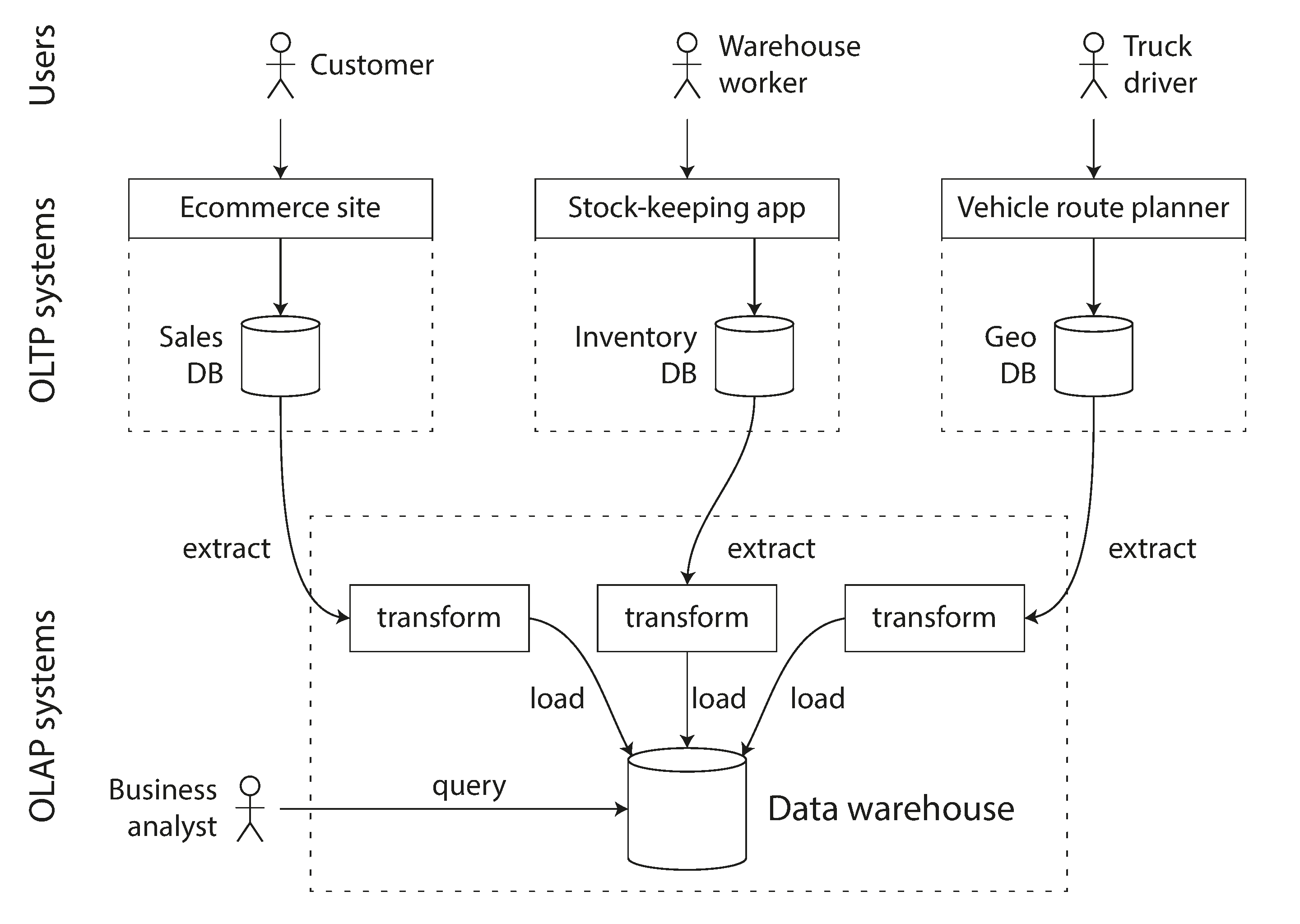
Data Warehousing

• A data warehouse, by contrast, is a separate database that analysts can query to their hearts’ content, without affecting OLTP operations. The data warehouse contains a read-only copy of the data in all the various OLTP.
• The process of getting data into the warehouse is known as Extract–Transform–Load (ETL).

On the surface, a data warehouse and a relational OLTP database look similar, because they both have a SQL query interface. However, the internals of the systems can look quite different, because they are optimized for very different query patterns.

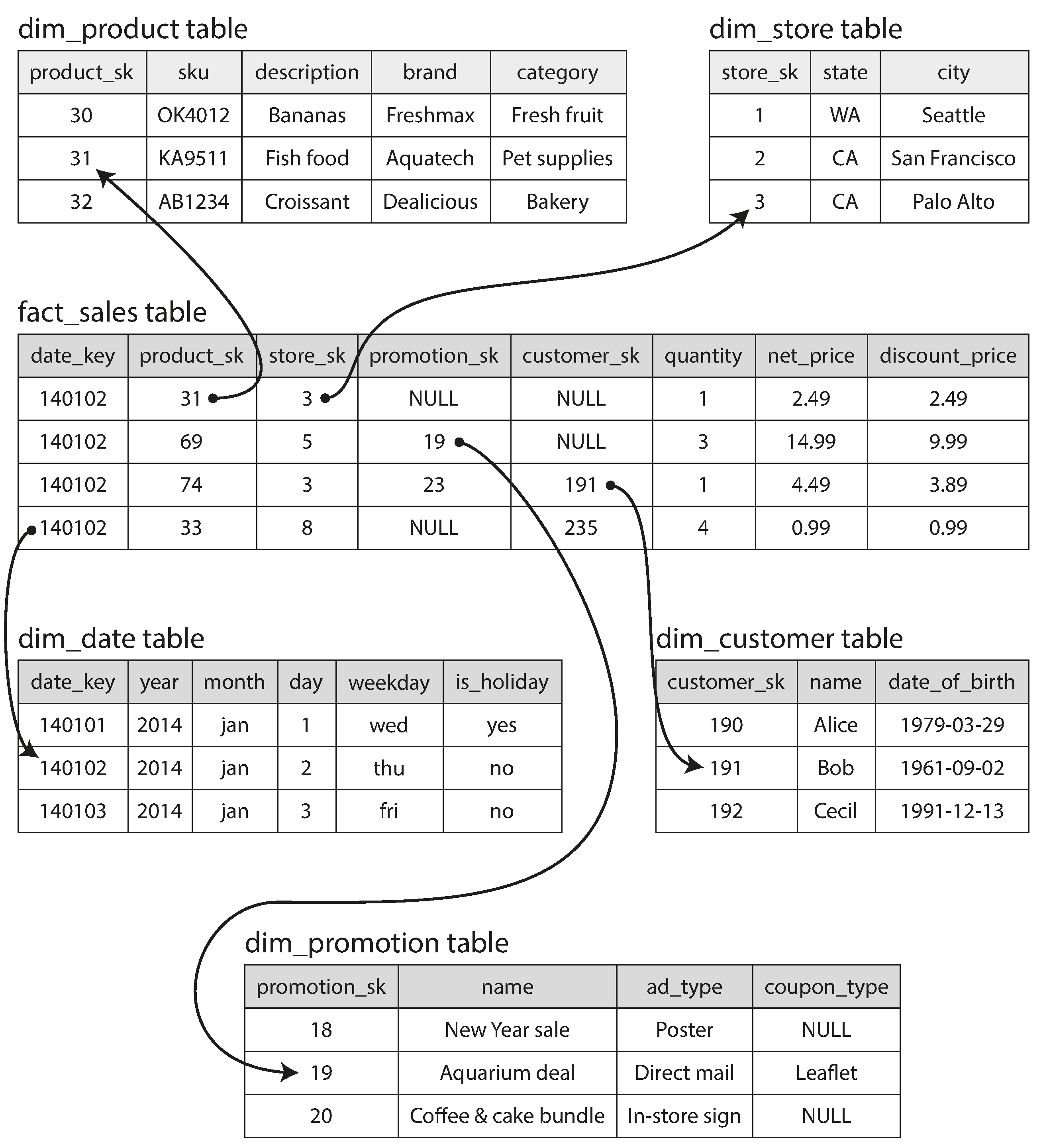
Stars and Snowflakes: Schemas for Analytics

• Many data warehouses are used in a fairly formulaic style, known as a star schema (also known as dimensional modeling ).
• At the center of the schema is a so-called fact table.
• Other columns in the fact table are foreign key references to other tables, called dimension tables. As each row in the fact table represents an event, the dimensions represent the who, what, where, when, how, and why of the event.
• A variation of this template is known as the snowflake schema, where dimensions are further broken down into subdimensions.

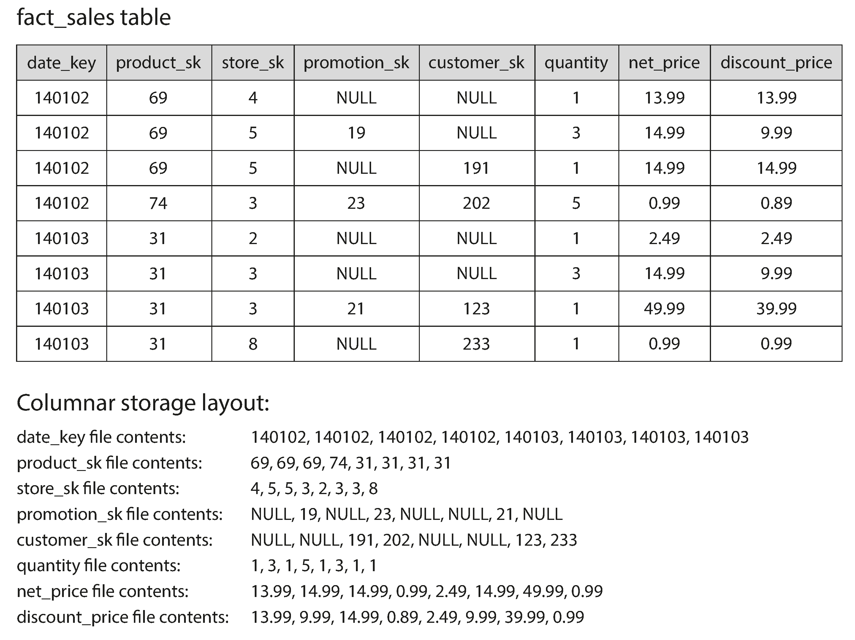
Column-Oriented Storage

The idea behind column-oriented storage is simple: don’t store all the values from one row together, but store all the values from each column together instead. If each column is stored in a separate file, a query only needs to read and parse those columns that are used in that query, which can save a lot of work.

Column Compression

bitmap encoding

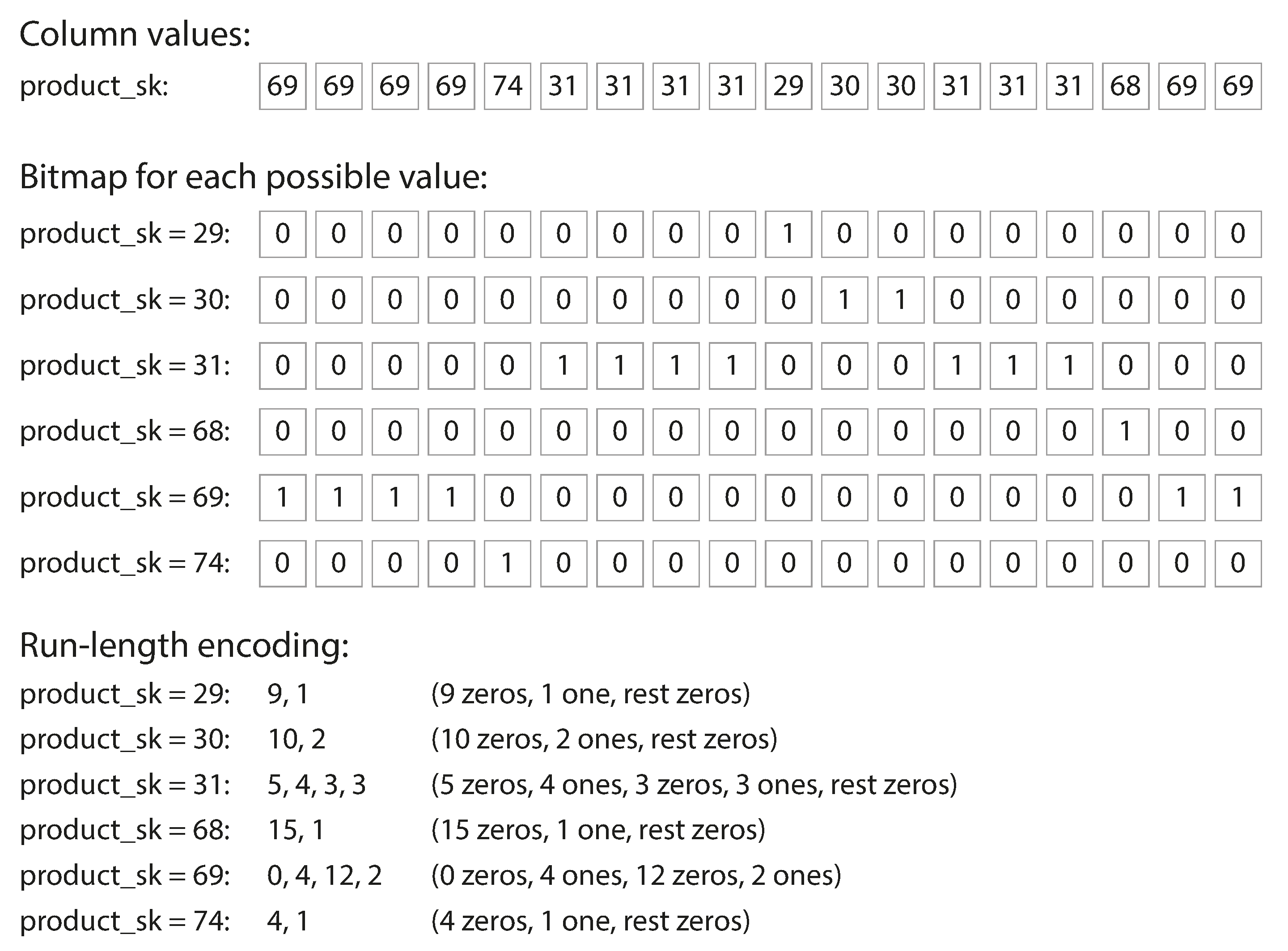
Operators, such as the bitwise AND and OR described previously, can be designed to operate on such chunks of compressed column data directly. This technique is known as vectorized processing.

Several different sort orders

Vertica store data in multiple sorted order, use the version that best fits the query.

Writing to Column-Oriented Storage

Use LSM-trees. All writes first go to an in-memory store, where they are added to a sorted structure and prepared for writing to disk. It doesn’t matter whether the in-memory store is row-oriented or column-oriented. When enough writes have accumulated, they are merged with the column files on disk and written to new files in bulk. This is essentially what Vertica does.

Aggregation: Data Cubes and Materialized Views

• materialized view is an actual copy of the query results, written to disk, whereas
• a virtual view is just a shortcut for writing queries

materialized view is used more in read heavy OLAP systems, since it needs to be updated when write happens.

A common special case of a materialized view is known as a data cube or OLAP cube.

Summary

On a high level, we saw that storage engines fall into two broad categories:

• those optimized for transaction processing (OLTP),
• and those optimized for analytics (OLAP).

There are big differences between the access patterns in those use cases:

1. OLTP systems are typically user-facing, which means that they may see a huge volume of requests.
   • In order to handle the load, applications usually only touch a small number of records in each query.
   • The application requests records using some kind of key, and the storage engine uses an index to find the data for the requested key.
   • Disk seek time is often the bottleneck here.
2. Data warehouses and similar analytic systems are less well known, because they are primarily used by business analysts, not by end users.
   • They handle a much lower volume of queries than OLTP systems, but each query is typically very demanding, requiring many millions of records to be scanned in a short time.
   • Disk bandwidth (not seek time) is often the bottleneck here, and columnoriented storage is an increasingly popular solution for this kind of workload.

On the OLTP side, we saw storage engines from two main schools of thought:

1. The log-structured school,
   • which only permits appending to files and deleting obsolete files, but never updates a file that has been written. + + Bitcask, SSTables, LSM-trees, LevelDB, Cassandra, HBase, Lucene, and others belong to this group.
2. The update-in-place school,
   • which treats the disk as a set of fixed-size pages that can be overwritten.
   • B-trees are the biggest example of this philosophy, being used in all major relational databases and also many nonrelational ones.

Log-structured storage engines are a comparatively recent development. Their key idea is that they systematically turn random-access writes into sequential writes on disk, which enables higher write throughput due to the performance characteristics of hard drives and SSDs.