Natural Language Processing
Notes taken for self studying Stanford CS224N
1. Introduction to Natural Language Processing
What is Natural Language Processing?
Natural Language Processing (NLP) is the development and study of automatic systems that understand and generate natural (human) languages.
Key Characteristics of Natural Language:
- Discrete/symbolic/categorical system: Words are symbols with meaning
- Signifier-signified relationship: Words (signifiers) map to ideas or things (signified)
- Multi-modal encoding: Language symbols can be expressed through voice, gesture, writing, etc.
- Continuous signal transmission: These symbols are transmitted as continuous signals to the brain
NLP Task Difficulty Hierarchy
Easy Tasks:
- Spell checking
- Keyword search
- Finding synonyms
Medium Tasks:
- Parsing information from websites and documents
- Information extraction
Hard Tasks:
- Machine translation
- Semantic analysis
- Coreference resolution
- Question answering
Word Representation
- Core principle: Words must be represented as vectors to enable computational processing
- Similarity requirement: To perform well on NLP tasks, we need quantifiable notions of similarity and difference between words
- Distance measures: Jaccard, Cosine, Euclidean distances help measure word relationships
2. Word Vectors
The Vector Space Hypothesis
- Goal: Encode word tokens as vectors representing points in a semantic “word space”
- Dimensionality assumption: There exists an N-dimensional space where \(N \ll Size(vocabulary)\) that can encode all language semantics
- Semantic dimensions: Each dimension encodes meaningful linguistic properties (tense, count, gender, etc.)
One-Hot Vectors
Definition: Represent every word as an \(\mathbb{R}^{\vert V \vert \times 1}\) vector with all zeros and a single one
Problems with one-hot vectors
- No notion of similarity (all dot products = 0)
- Extremely sparse representation
- Vocabulary-dependent dimensionality
3. SVD-Based Methods
Core Approach
- Data collection: Loop over corpus and accumulate word co-occurrence counts in matrix \(X\)
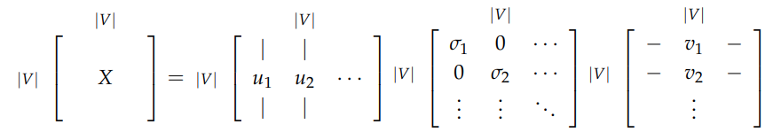
- Decomposition: Perform Singular Value Decomposition: \(X=USV^T\)
- Embedding extraction: Use rows of \(U\) as word embeddings
3.1 Word-Document Matrix
Assumption: Related words often appear in the same documents
Structure:
- Matrix \(X \in \mathbb{R}^{\vert V \vert \times M}\) (Vocabulary x Document)
- Also known as document-term matrix
- Scales with number of documents M
3.2 Window-Based Co-occurrence Matrix
Assumption: Related words appear close to each other in text
Structure:
- Matrix \(X \in \mathbb{R}^{\vert V \vert \times \vert V \vert}\) (Vocabulary x Vocabulary)
- \(X\) is an affinity matrix counting co-occurrences within a fixed window
- Fixed size based on vocabulary, window size is hyperparameter
3.3 SVD Application Process
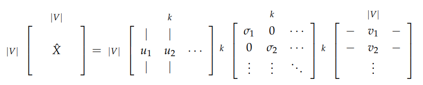
- Rank selection: Examine diagonal values in \(S\) matrix
- Dimensionality reduction: Cut off at index \(k\) based on desired variance captured
- Embedding extraction: Select first \(k\) columns of \(U\) as word vectors
SVD Method Limitations
Major Problems:
Both of these methods give us word vectors that are more than sufficient to encode semantic and syntactic (part of speech) information but are associated with many other problems:
- Dynamic dimensionality: Matrix dimensions change frequently (new words, documents)
- Extreme sparsity: Most words don’t co-occur
- High dimensionality: Matrices can be \(\approx 10 ^6\times 10^6\)
- Computational cost: Quadratic training time (SVD)
- Frequency imbalance: Requires hacks like TF-IDF or BM25
Partial Solutions:
- Filter function words (“the”, “he”, “has”, etc.)
- Apply ramp window weighting based on word distance
- Use Pearson correlation, set negative counts to zero
Iteration based methods solve many of these issues.
4. Iterative Methods - Word2Vec
Core Philosophy
Instead of computing global corpus information, create models that:
- Learn iteratively, one step at a time
- Encode probability of words given their context
- Use distributional similarity assumption: similar words have similar contexts
Word2Vec Components
Two Algorithms:
- CBOW (Continuous Bag of Words): Predicts center word from surrounding context
- Skip-gram: Predicts context words from center word
Two Training Methods:
- Negative sampling: Defines objective by sampling negative examples
- Hierarchical softmax: Uses efficient tree structure for probability computation
4.1 Language Models
Unigram Model (independence assumption):
\[P(w_1, w_2, ..., w_n) = \prod_{i=1}^{n}P(w_i)\]Bigram Model (pairwise dependency):
\[P(w_1,w_2,...,w_n) = \prod_{i=2}^{n}P(w_i \vert w_{i-1})\]4.2 Continuous Bag of Words (CBOW)
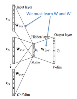
Objective: Given context words {“The”, “cat”, “over”, “the”, “puddle”}, predict center word “jumped”
Architecture:
- Two parameter matrices:
- \(\mathit{V} \in \mathbb{R}^{n \times \vert V \vert}\) (context word vectors)
- \(\mathit{U} \in \mathbb{R}^{\vert V \vert \times n}\) (center word vectors)
Forward Pass Process:
- Input: One-hot context vectors \((x^{c-m},...,x^{c-1},x^{c+1},...,x^{c+m})\)
- Embedding lookup: Context vectors \((v_{c-m}=Vx^{c-m},...,v_{c+m}=Vx^{c+m})\)
- Averaging: \(\hat{v} = \frac{v_{c-m}+v_{c-m+1}+...+v_{c+m}}{2m}\)
- Scoring: \(z=U\cdot\hat{v} \in \mathbb{R}^{\vert V \vert}\) As the dot product of similar vectors is higher, it will push similar words close to each other(ideally predicted center word and true center word) in order to achieve a high score.
- Probability: \(\hat{y} \in \mathbb{R}^{\vert V \vert} = softmax(z)\), where \(softmax(v) = \frac{e^{v_i}}{\Sigma_{k=1}^{\vert V \vert}e^{y_k}} \quad for \qquad i \in \vert V \vert\)
- Target: We want the predicted probabilities to match the true probabilities, \(y\in\mathbb{R}^{\vert V \vert}\) which is the one-hot encoded center word.
Loss function:
- Cross entropy:
It gives us a good measure of distance.
Objective Function:
\[\begin{align} minimize J &=-logP(w_c \vert w_{c-m},...,w_{c+m}) \\ &= -logP(u_c\vert \hat{v}) \\ &= -log\frac{exp(u_c^T\hat{v})}{\Sigma_{j=1}^{\vert V \vert}exp(u_j^T\hat{v})} \\ &= -u_c^T\hat{v} + log\Sigma_{j=1}^{\vert V \vert}exp(u_j^T\hat{v}) \end{align}\]Optimization: Stochastic Gradient Descent (SGD).
- \[U\leftarrow U-\alpha\nabla _uJ; V\leftarrow V-\alpha\nabla_vJ\]
4.3 Skip-Gram Model
Objective: Given center word “jumped”, predict context words
Key Difference: Swaps input and output compared to CBOW
Forward Pass Process:
- Input: One-hot center word vector \(x\in\mathbb{R}^{\vert V \vert}\)
- Embedding Lookup: \(v_c=V_x\in\mathbb{R}^n\)
- Scoring: \(z=Uv_c\in \mathbb{R}^{\vert V \vert}\)
- Probability: \(\hat{y} = softmax(z)\)
- Target: Context word one-hot vectors \(y^{c-m},...,y^{c+m}\)
Naive Bayes Assumption: All output words are conditionally independent
Objective Function:
\[\begin{align} minimize J &=-logP(w_{c-m}, ..., w_{c+m}|w_c) \\ &= -log\prod_{j=0,j\neq m}^{2m}P(w_{c-m+j} \vert w_c) \\ &= -log\prod_{j=0,j\neq m}^{2m}P(u_{c-m+j} \vert v_c) \\ &= -log\prod_{j=0,j\neq m}^{2m}\frac{exp(u_{c-m+j}^Tv_c)}{\sum_{k=1}^{\vert V \vert}exp(u_{k}^Tv_c)} \\ &= -\sum_{j=0,j\neq m}^{2m}u_{c-m+k}^Tv_c+2mlog\sum_{k=1}^{\vert V \vert}exp(u_k^Tv_c) \end{align}\]Alternative Formulation:
\[J=-\sum_{j=0,j\neq m}^{2m}logP(u_{c-m+j}|v_c) = \sum_{j=0,j\neq m}^{2m}H(\hat{y}, y_{c-m+j})\]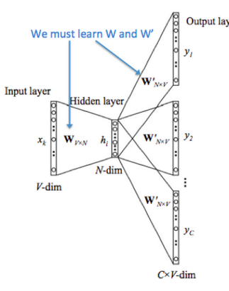
4.4 Negative Sampling
Problem: Objective function requires summation over entire vocabulary \(\vert V \vert\).
Solution: Approximate by sampling negative examples from noise distribution \(P_n(w)\) whose probabilities match the ordering of the frequency of the vocabulary
Approach: For word-context \((w, c)\), define:
- \(P(D=1 \vert w,c)\): Probability pair came from real data
- \(P(D=0 \vert w,c)\): Probability pair is synthetic/negative
Model:
\[P(D=1 \vert w,c) = \sigma(v_c^Tv_w) = \frac{1}{1+ e^(-v_c^Tv_w)}\]Maximum Likelihood Estimation:
\[\begin{align} \theta &= \underset{\theta}{argmax} \prod_{(w,c)\in D} P(D=1|w,c,\theta)\prod_{(w,c)\in \tilde{D}} P(D=0|w,c,\theta) \\ &= \underset{\theta}{argmax} \prod_{(w,c)\in D} P(D=1|w,c,\theta) \prod_{(w,c)\in \tilde{D}}(1-P(D=1 \vert w,c,\theta)) \\ &= \underset{\theta}{argmax} \sum_{(w,c)\in D}logP(D=1|w,c,\theta) + \sum_{(w,c)\in\tilde{D}}log(1-P(D=1 \vert w, c,\theta)) \\ &= \underset{\theta}{argmax} \sum_{(w,c)\in D}log\frac{1}{1+exp(-u_w^Tv_c)} + \sum_{(w,c)\in\tilde{D}}log(1-\frac{1}{1+exp(-u_w^Tv_c)}) \\ &= \underset{\theta}{argmax} \sum_{(w,c)\in D}log\frac{1}{1+exp(-u_w^Tv_c)} + \sum_{(w,c)\in\tilde{D}}log(\frac{1}{1+exp(u_w^Tv_c)}) \\ \end{align}\]Objective Function: Maximizing the likelihood is the same as minimizing the negative log likelihood.
\[J=-\sum_{(w,c)\in D}log\frac{1}{1+exp(-u_w^Tv_c)} - \sum_{(w,c)\in\tilde{D}}log(\frac{1}{1+exp(u_w^Tv_c)})\]\(\tilde{D}\) is false for negative corpus, we can generate on the fly by randomly sampling from the word bank.
Skip-gram with Negative Sampling:
\[-log\sigma(u_{c-m+j}^T\cdot v_c)-\sum_{k=1}^{K}log\sigma(-\tilde{u}_k^T\cdot v_c)\]CBOW with Negative Sampling:
\[-log\sigma(u_c^T\cdot\hat{v}) - \sum_{k=1}^{K}log\sigma(-\tilde{u}_k^T\cdot \hat{v})\]Noise Distribution: Unigram model rasisd to power of 3/4 works best emperically. \(P_n(w) \propto U(w)^{\frac{3}/{4}}\\)
4.5 Hierarchical Softmax
Purpose: Efficient alternative standard softmax
When to Use:
- Hierarchical softmax: Better for infrequent words
- Negative sampling: Better for frequent words and lower-dimensional vectors
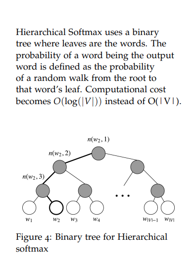
Structure:
- Binary tree representing entire vocabulary
- Each leaf is a a word, unique root-to-leaf path
- Internal nodes have learned vector representations
- No output word representations needed
Probability Computation: The probability of a word \(w\) given a vector \(w_i\), \(p(w \vert w_i)\) is equal to the probability of a random walk starting in the root and ending in the lead node corresponding to \(w\).
\[P(w \vert w_i)=\prod_{j=1}^{L(w)-1}\sigma([n(w, j+1)=ch(n(w,j))]\cdot v_{n(w,j)}^Tv_{w_i})\]where:
- \([x] = 1\) if \(x\) is true, \(-1\) otherwise
- \(n(w, i)\) is the i-th node from root to w
- \(ch(n)\): left children of node \(n\)
- \(L(w)\): path length to word \(w\)
- \([n(w, j+1)=ch(n(w,j))]\) will be 1 if node is left -1 if node is right, thus ensures proper normalization.
Computational Complexity: \(O(log(\vert V \vert))\)
Training: Minimize the negative log-likelihood by updating internal node vectors binary tree
5. Key Takeaways
- Evolution: NLP word representation evolved from sparse one-hot vectors → SVD-based dense vectors → Iterative learned
- Trade-offs:
- SVD: Global optimization but computational challenges
- Word2Vec: Efficient iterative learning but local optimization
- Context Matters: Both CBOW and Skip-gram leverage distributional hypothesis that similar words appear in similar contexts
- Efficiency Solutions: Negative sampling and hierarchical softmax address computational bottlenecks in neural language models
6 Global Vectors for Word Representation (GloVe)
1.1 Comparison with Previous Methods
- Count based
- Rely on Matrix factorization. (LSA, HAL)
- Effectively leverage global statistical information
- Ok with word similarities, but poorly on other tasks -> vector space structure is sub-optimal.
- Shallow window-based
- Skip-gram and CBOW
- Learn embedding by making predictions in local context windows
- Capture complex linguistic patterns beyond word similarity
- Fail to make use of the global co-occurrence statistics
- GolVe
- Using global statistics to predict the probability of word pair co-occurrence
1.2 Co-occurrence Matrix
- \(X_{ij}\) indicates the number of time word \(j\) occur in the context of word \(i\)
- \(X_i=\sum_kX_{ik}\) be the number of times any word \(k\) appears in the context of word \(i\)
- \(P_{ij} = p(w_j \vert w_i) = \frac{X_{ij}}{X_{i}}\) is the probability of \(j\) appearing in the context of word \(i\)
1.3 Least Squares Objective
-
softmax compute the probability of word \(j\) appears in the context of word \(i\)
\[Q_{ij} = \frac{exp(u_j^Tv_i)}{\sum_{w=1}^{W}exp(u_w^Tv_i)}\] -
Global corss-entropy objective function trained in an on-line, stochastic fashion
\[J = -\sum_{i \in \text{corpus}}\sum_{j \in \text{context(i)}}logQ_{ij}\] -
It is more efficient to group together the same values for \(i\) and \(j\)
\[J=-\sum_{i=1}^{W}\sum_{j=1}^{W}X_{ij}logQ_{ij}\]where the value of co-occurring frequency is given by the co-occurrence matrix X
- One drawback of the cross-entropy loss is that it requires the distribution \(Q\) to be properly normalized, which involves the expensive summation over the entire vocabulary.
-
Instead, we use a least square objective in which the normalization factors in \(P\) and \(Q\) are discarded:
\[\hat{J}=\sum_{i=1}^{W}\sum_{j=1}^{W}X_{ij}(\hat{P_{ij}}-\hat{Q_{ij}})^2\]where \(\hat{P_{ij}} = X_{ij}\) and \(\hat{Q_{ij}} = exp(u_j^Tv_i)\) are the unnormalized distributions.
- New problem: \(X_{ij}\) often takes on very large values and makes the optimization difficult.
-
Solution: minimize the squared error of the logarithm of \(\hat{P}\) and \(\hat{Q}\)
\[\begin{align} \hat{J} &= \sum_{i=1}^{W} \sum_{j=1}^{W}X_i(log(\hat{P_{ij}}) - log(\hat{Q_{ij}}))^2\\ &=\sum_{i=1}^{W} \sum_{j=1}^{W}X_i(u_j^Tv_i - logX_{ij})^2 \\ &=\sum_{i=1}^{W} \sum_{j=1}^{W}f(X_{ij})(u_j^Tv_i - logX_{ij})^2 \end{align}\]where \(f(X_{ij})\) is a more general weighting function than the raw \(X_i\)
7 Evaluation of Word Vectors
2.1 Intrinsic Evaluation
- Evaluate word vectors on specific intermediate subtasks. Like analogy completion for question answering. Reason? If evaluated with the final downstream task, the entire pipeline will be retrained from scratch each time we need to tweak the word vector learning.
- Requirement: the intrinsic evaluation has a positive correlation with the final task performance.
2.2 Extrinsic Evaluation
- Evaluate word vectors on the real task.
- Typically, optimizing over an under performing extrinsic evaluation system does not allow us to determine which specific subsystem is at fault and this motivates the need for intrinsic evaluation.
2.3 Intrinsic Evaluation Example: Word Vector Analogies
-
a:b::c:? -
find \(d\) such that it maximizes the cosine similarity
\[d=\underset{i}{argmax}\frac{(x_b-x_a+x_c)^Tx_i}{||x_b-x_a+x_c||}\] -
semantic: capital city -> country
-
syntactic: adj -> it’s superlative form
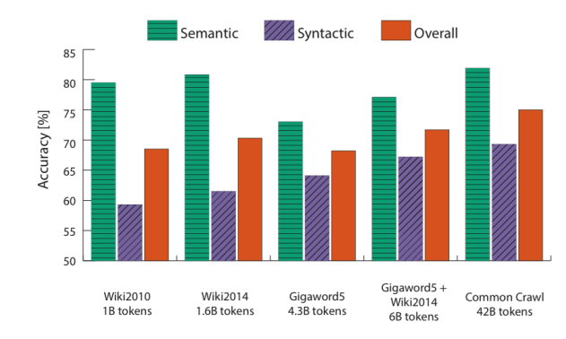
2.4 Analogy Evaluations
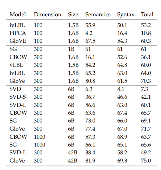
- Performance is heavily dependent on the model used for word embedding.
- Performance increases with larger corpus sizes
- Performance is lower for extremely low dimensional word vectors
- Extremely high dimensional vectors with CBOW/SG is reasonably robust to noise
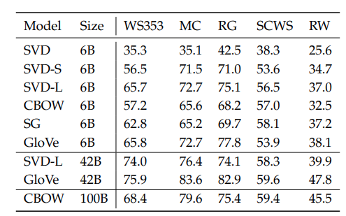
2.5 Correlation Evaluation
- Another simple way to evaluate the quality of word vectors is by asking humans to assess the similarity between two words on a fixed scale and then comparing this with the cosine similairity between the corresponding word vectors.
2.6 Dealing With Ambiguity
- Improving word representations via global context and multiple word prototypes. Huang et.al. 2012
8. Training for Extrinsic Tasks
3.1 Problem Formulation
- Most NLP extrinsic tasks can be formulated as classification tasks.
- Sentiment analysis: given a text, classify it to be negative or positive.
- Named-entity recognition(NER): given a context and a center word, classify the center word to be one of many classes.
3.2 Retraining Word Vectors
- If we retrain word vectors using the extrinsic task, we need to ensure that the training set is large enough to cover most words from the vocabulary.
- When retrain word vectors over a small set of the vocabulary, these words are shifted in the word space and as a result, the performance over the final task could actually reduce.
3.3 Softmax Classification and Regularization
-
Softmax classification:
\[p(y_j=1|x) = \frac{exp(W_j\cdot x)}{\sum_{c=1}^{C}exp(W_c\cdot x)}\] -
Using the cross-entropy loss:
\[-\sum_{j=1}^{C}y_jlog(p(y_j=1|x)) = -\sum_{j=1}^{C}y_j log(\frac{exp(W_j\cdot x)}{\sum_{c=1}^{C}exp(W_c\cdot x)})\] -
Since there is only one correct answer, let $k$ be the correct one. The loss function simplify to:
\[-log(\frac{exp(W_k\cdot x)}{\sum_{c=1}^{C}exp(W_c\cdot x)})\] -
Extend to a dataset of N points:
\[-\sum_{i=1}^{N}log(\frac{exp(W_{k(i)}\cdot x^{(i)})}{\sum_{c=1}^{C}exp(W_c\cdot x^{(i)})})\] -
We have \(C\cdot d+\vert V \vert\cdot d\) parameters to update each time. To avoid, over fitting, we can pose the Bayesian belief that parameters \((\theta)\) should be small in magnitude:
\[-\sum_{i=1}^{N}log(\frac{exp(W_{k(i)}\cdot x^{(i)})}{\sum_{c=1}^{C}exp(W_c\cdot x^{(i)})}) + \lambda \sum_{k=1}^{C\cdot d + \vert V \vert\cdot d}{\theta_k}^2\]
3.4 Window Classification
- Instead of using just the word of interest, use a sequence that is a center word preceded and suceeded by context words.
- Generally, narrower window sizes lead to better performance in syntactic tests while wider windows lead to better performance in semantic tests.
3.5 Non-linear Classifiers
- Non-linear decision boundaries to solve not linear separable classification problem.
9 Dependency Grammar and Dependency Structure
- Parse trees in NLP are used to analyze the syntactic structure of sentences.
- Constituency structures - phrase structure grammar to organize words into nested constituents.
- Dependency structures - shows which words depend on (modify or are argument of) which other words.
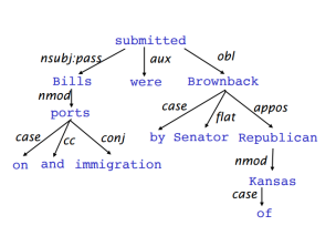
- Dependency tree for the sentence: “Bills on ports and immigration were submitted by Senator Brownback, Republican of Kansas.”
1.1 Dependency Parsing
- Task of analyzing the syntactic dependency structure of a given input sentence S.
- Output is a dependency tree/graph \(G\) where the words are connected by typed dependency relations.
- Learning: Given a training set \(D\) of sentences annotated with dependency graphs, induce a parsing model M that can be used to parse new sentences.
- Parsing: Given a parsing model M and a sentence S, derive the optimal dependency graph D for S according to M.
1.2 Transition-Based Dependency Parsing
- State machine which defines the possible transitions to create the mapping from the input sentence to the dependency tree.
- Learning: induce a model to predict the next transition
- Parsing: construct the optimal sequence of transitions
- Most transition-based systems do not make use of a formal grammar.
1.3 Greedy Deterministic Transition-Based Parsing
-
Nivra 2003, showed to be better in both performance and efficiency than traditional feature-based discriminative dependency parsers.
- States:
- For any sentence \(S=w_0w_1...w_n\) a state can be described with a triple \(c=(\sigma, \beta,A)\)
- a stack \(\sigma\) of words \(w_i\) from \(S\)
- a buffer \(\beta\) of words \(w_i\) from \(S\)
- a set of dependency arcs \(A\) of the form \((w_i, r, w_j)\), where \(w_i, w_j\) are from \(S\), and \(r\) describes a dependency relation.
- It follows that for any sentence \(S=w_0w_1...w_n\),
- an initial state \(c_0\) is of the form \((\vert w_0 \vert _{\sigma}, [w_1,...,w_n]_{\beta}, \emptyset)\)
- a terminal state has the form \((_{\sigma}, []_{\beta}, A)\)
- For any sentence \(S=w_0w_1...w_n\) a state can be described with a triple \(c=(\sigma, \beta,A)\)
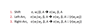
- Transitions
- SHIFT: remove the first word in the buffer and push it on top of the stack
- LEFT-ARC: add a dependency arc \((w_j, r, w_i)\) to the arc set \(A\), where \(w_i\) is the word second to the top of the stack and \(w_j\) is the word at the top of the stack. Remove \(w_i\) from the stack
- RIGHT-ARC: dd a dependency arc \((w_i, r, w_j)\) to the arc set A, where \(w_i\) is the word second to the top of the stack and \(w_j\) is the word at the top of the stack. Remove \(w_j\) from the stack
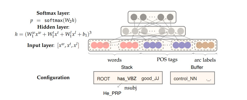
1.4 Neural Dependency Parsing
- Feature Selection:
- \(S_{word}\) vector representations for some of the words in \(S\) (and their dependents) at the top of the stack \(\sigma\) and buffer \(\beta\)
- \(S_{tag}\): Part-of-Speech (POS) tags for some of the words in \(S\). POS tags comprise a small, discrete set: \(P=\{NN,NNP,NNS,DT,JJ,...\}\)
- \(S_{label}\): The arc-labels for some of the words in \(S\). The arc-labels comprise a small discrete set, describing the dependency relation: \(L=\{amod, tmod,nsubj,csubj,dobj,...\}\)
- For each feature type, we will have a corresponding embedding matrix, mapping from the feature’s one hot encoding , to a \(d-\) dimensional dense vector representation.
- For example:
- \(S_{word}\): top 3 words on stack and buffer, the first and second leftmost / right most children of the top two words on the stack. the leftmost of leftmost / rightmost of rightmost children of the top two words on the stack. 18 elements in total
- \(S_{tag}\): 18 corresponding tags
- \(S_{label}\): 12 in total.
- Model:
10 Language Models
1.1 Introduction
-
Language models compute the probability of occurrence of a number of words in a particular sequence.
-
The probability of a sequence of \(m\) words \(\{w_1, ..., w_m\}\) is \(P(w_1,...,w_m)\)
-
It is usually conditioned on a window of \(n\) previous words rather than all previous words:
\[P(w_1, ..., w_m) = \prod_{i=1}^{m}P(w_i \vert w_1,...,w_{i-1}) \approx \prod_{i=1}^{m}P(w_i \vert w_{i-n},...,w_{i-1})\]
1.2 n-gram Language Models
-
One way to compute the above probabilities is n-gram.
-
Bigram: \(p(w_w \vert w_1) = \frac{count(w_1, w_2)}{count(w_1)}\)
-
Trigram: \(p(w_3 \vert w_1,w_2) = \frac{count(w_1, w_2, w_3)}{count(w_1, w_2)}\)
-
Main issues with n-gram Language Models:
- Sparsity problems:
- If \(w_1, w_2\) never appear together, the numerator for trigram is 0. Add smoothing a small \(\delta\).
- If \(w_1, w_2\) never appear together, the denominator for trigram is 0. Can condition on \(w_2\) alone, called backoff.
- Increasing \(n\) makes sparsity problems worse. Typically, \(n\leq 5\)
- Storage problems with n-gram Language Models:
- Store counts for all n-grams is large and it grow fast as corpus size grows.
- Sparsity problems:
1.3 Window-based Neural Language Model
- Bengio et al Neural Probabilistic Language Model, first large-scale deep learning for natural language processing model.
- It learns a distributed representation of words, along with the probability function for word sequences expressed in terms of these representations.
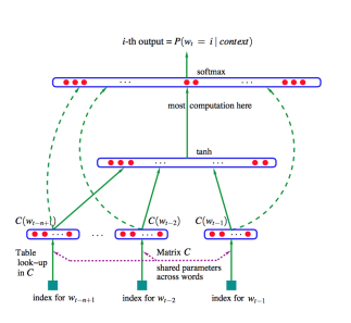
- Consider window-based model as Language Model conditioned on fixed size history of information.
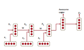
11 Recurrent Neural Networks (RNN)
- RNN can conditioning the Language Model on all previous words.
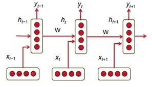 \(h_t = \sigma(W^{(hh)}h_{t-1}+W^{(hx)}x_{[t]}) \\
\hat{y}_t = softmax(W^{(S)}h_t)\)
\(h_t = \sigma(W^{(hh)}h_{t-1}+W^{(hx)}x_{[t]}) \\
\hat{y}_t = softmax(W^{(S)}h_t)\)
- \(W^{(hh)}\) and \(W^{(hx)}\) are shared across time, applied repeatedly at each step.
- Thus model learn fewer parameters
- And is independent of the length of the input sequence
- Defeating the curse of dimensionality
2.1 RNN Loss and Perplexity
- RNN trained with cross entropy loss
-
At a given time \(t\) the loss is
\[J^{(t)}(\theta) = -\sum_{j=1}^{\vert V \vert}y_{t,j} \times log(\hat{y}_{t,j})\] -
Aggregate over the corpus:
\[J = \frac{1}{T}\sum_{t=1}^{T}J^{(t)}(\theta) = -\frac{1}{T}\sum_{t=1}^{T}\sum_{j=1}^{\vert V \vert}y_{t.j} \times log(\hat{y}_{t, j})\] -
The perplexity is defined as: \(2^{J}\)
Lower value imply more confident in predicting the next word in sequence
2.2 Advantages, Disadvantages and Applications of RNNs
- Advantages:
- process input sequences of any length
- model size independent of sequence lengths
- computation for step \(t\) can (in theory) use information from many steps back
- Disadvantages:
- computation is slow - because it is sequential, can’t be parallelized
- in practice, it is difficult to access information from many steps back due to vanishing and exploding gradients.
- RNNs can be used for many tasks, such as tagging (POS, NER), sentence classification(category, sentiment), and as encoder or decoder modules.
2.3 Vanishing Gradient & Gradient Explosion Problems
\[\begin{align} \frac{\partial E}{\partial W} &= \sum_{t=1}^{T}\frac{\partial E_t}{\partial W} \\ \frac{\partial E_t}{\partial W} &= \sum_{k=1}^{t}\frac{\partial E_t}{\partial y_t}\frac{\partial y_t}{\partial h_t}\frac{\partial h_t}{\partial h_k}\frac{\partial h_k}{\partial W} \\ \frac{\partial h_t}{\partial h_k} &= \prod_{j=k+1}^{t}\frac{\partial h_{j}}{\partial h_{j-1}}=\prod_{j=k+1}^{t}W^T \times diag[f'(j_j-1)] \\ \frac{\partial E}{\partial W} &= \sum_{t=1}^{T}\sum_{k=1}^{t}\frac{\partial E_t}{\partial y_t}\frac{\partial y_t}{\partial h_t}(\prod_{j=k+1}^{t}\frac{\partial h_j}{\partial h_{j-1}})\frac{\partial h_k}{\partial W} \end{align}\]\(\partial h_{j} / \partial h_{j-1}\) is the Jacobian matrix for h.
\[\|\frac{\partial h_j}{\partial h_{j-1}}\| \leq \|W^T\| \|diag[f'(h_{j-1})] \| \leq \beta_W \beta_h\]Where \(\beta_W\) and \(\beta_h\) are the upper bound values for the norms of the two matrices. \(f'(h_{j-1})\) can only be as large as 1, given sigmoid activation.
\[\|\frac{\partial h_t}{\partial h_k}\| = \| \prod_{\partial h_{j-1}}^{\partial h_{j}} \| \leq (\beta_W\beta_h)^{t-k}\]- if \(\beta_W\beta_h\) get smaller or larger than 1, with \(t-k\) sufficiently large, the gradients blows or diminishes very quickly.
- Gradient Explosion, i.e. gradient overflow the floating number limits becomes NaN, can be detected.
- Gradient Vanish, i.e. gradient becomes 0, can be undetected. It will be hard to tell whether it is that:
- No relationship last that long, or
- We can’t capture this due to gradient vanishing.
2.4 Solution to the Exploding & Vanishing Gradients
-
For exploding gradient: gradient clipping
\[\hat{g} \leftarrow \frac{\partial E}{\partial W} \\ if \quad \|\hat{g}\| \geq threshold \quad then \\ \hat{g} \leftarrow \frac{threshold}{\|\hat{g}\|}\hat{g}\] -
For vanishing gradient:
- identity matrix initialization
- use ReLU activations
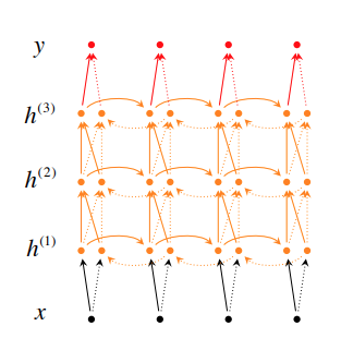
2.5 Deep Bidirectional RNNs
-
Bidirectional
\[\begin{align} \overrightarrow{h_t} &= f(\overrightarrow{w_{x_t}} + \overrightarrow{V} \, \, \, \overrightarrow{h}_{t-1} + \overrightarrow{b}) \\ \overleftarrow{h_t} &= f(\overleftarrow{w_{x_t}} + \overleftarrow{V} \, \, \, \overleftarrow{h}_{t-1} + \overleftarrow{b}) \\ \hat{y}_t &= g(Uh_t + c) = g(U[\overrightarrow{h}_t; \overleftarrow(h)_t] + c) \end{align}\] -
Stacked RNN
\[\overrightarrow{h}^{(i)}_t = f(\overrightarrow{W}^{(i)} h^{(t-1)} + \overrightarrow{V}^{(i)} \overrightarrow{h}^{(i)}_{t-1} + \overrightarrow{b}^{(i)})\] -
The two can be combined
2.6 Application: RNN Translation Model
- Encoder-Decoder RNN for translation
- Encoder RNN process the input sequence and produce a final hidden state, that is feed into decoder RNN as the initial hidden state.
- The decoder RNN gets a
<BOS>token as initial input and treat each of the previous prediction as input to the current step.
- Extensions:
- Use dedicated Encoder and Decoder
- Use Bidirectional RNN
- Use Stacked RNN
- Compute every hidden state in the decoder using three inputs
- Previous hidden
- Previous step prediction
- Last hidden from encoder
- Sometimes worth trying instead of \(ABC\rightarrow XY\), do \(CBA\rightarrow XY\)
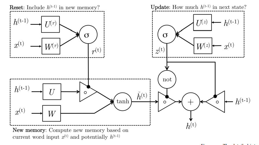
12 Gated Recurrent Units
- Although RNNs can theoretically capture long-term dependencies, they are very hard to actually train to do this.
-
Gated recurrent unites are designed in a manner to have more persistent memory thereby making it easier for RNNs to capture long-term dependencies.
\[\begin{align} \text{update gate} \qquad z_t &= \sigma(W^{(z)}x_t + U^{(z)}h_{t-1}) \\ \text{reset gate} \qquad r_t &= \sigma(W^{(r)}x_t + U^{(r)}h_{t-1}) \\ \text{new memory} \qquad \tilde{h}_t &= tanh(r_t\circ Uh_{t-1} + Wx_t) \\ \text{hidden state} \qquad h_t &= (1-z_t)\circ\tilde{h}_t+z_t\circ h_{t-1} \\ \end{align}\]
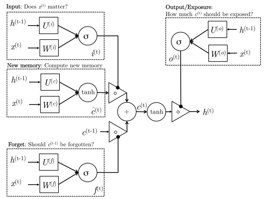
13 Long-Short-Term-Memories
- The motivation for LSTM is similar to GRU, the architecture of unit is a bit different.
-
LSTM has a separate cell state that is kept hidden. Hidden state is just a exposure of that cell state.
\[\begin{align} \text{input gate} \qquad i_t &= \sigma(W^{(i)}x_t + U^{(i)}h_{t-1}) \\ \text{forget gate} \qquad f_t &= \sigma(W^{(f)}x_t + U^{(f)}h_{t-1}) \\ \text{output gate} \qquad o_t &= \sigma(W^{(o)}x_t + U^{(o)}h_{t-1}) \\ \text{new memeory cell} \qquad \tilde{c}_t &= tanh(W^{(c)}x_t + U^{(c)}h_{t-1}) \\ \text{final state cell} \qquad c_t &= f_t \circ c_{t-1} + i_t\circ \tilde{c}_t \\ h_t &= o_t \circ tanh(c_t) \\ \end{align}\]
14 Statistical Machine Translation
-
probabilistic model and bayes rule:
\[argmax_yP(y \vert x) = argmax_yP(x \vert y)P(y)\] - where \(P(y)\) is the language model learned from monolingual data.
- and \(P(x \vert y)\) is the translation model learned from parallel data.
- Alignment - word-level correspondence between source sentence x and target sentence y
- decompose \(P(x \vert y)\) to \(P(x, a \vert y)\)
- alignments \(a\) are latent variables learned with EM algorithm.
- Dynamic programming is used for globally optimal solutions (Viterbi algorithm)
15 Neural Machine Translation with Seq2Seq
- Type of Seq2Seq usage:
- Translation
- Conversation
- Summarization
1.1 Brief Note on Historical Approaches
- Before neural network approach, translation systems were based on probabilistic models constructed from:
- a translation model, telling us what a sentence / phrase in a source language most likely translates into
- a language model, telling us how likely a given sentence / phrase is overall
- Phrase-based systems were most common prior to Seq2Seq. It is difficult to handle long-term dependencies with phrase-based system.
1.2 Sequence-to-sequence Basics
-
Appeared in 2014 for English-French translation
-
It is an end-to-end model made up of two RNNs:
- an encoder, which takes the model’s input sequence and encodes it into a fixed-size “context vector”
- an decoder, which uses the context vector from encoder as a “seed” from which to generate an output sequence.
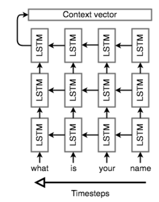
1.3 Seq2Seq architecture - encoder
- Use a encoder RNN to process the input token sequence and the final hidden state will become the context vector.
- Usually the Seq2Seq encoders will process the input sequence in reverse. It is done under the reasoning that the last thing the encoder sees will (roughly) corresponds to the first thing that the model ouputs. this makes it easier for the decoder to “get started”
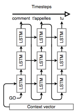
1.4 Seq2Seq architecture - decoder
- Use a decoder RNN to generate output sequence based of the words it generated so far, as well as the context.
- The decoding process is kicked off with a special token
<EOS>(if use the same RNN for both encoding and decoding) or<BOS>(If use dedicated networks)
- The decoding process is kicked off with a special token
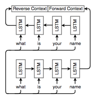
1.5 Bidirectional RNNs
- Use bidirectional RNNs to traversing a sequence in both directions and concatenating the resulting final hidden states and cell states.
16 Attention Mechanism
2.1 Motivation
- Bahdanau et al. 2016 proposing attention to address the issue with a single “context vector” for sequence-to-sequence models.
- Different parts of an input have different levels of significance
- Different parts of the output may consider different parts of the input “important”
- Attention mechanisms make use of this observation by providing the decoder network with a chance to look at the entire input sequence at every decoding step. The decoder can then decide what input words are important at any point in time.
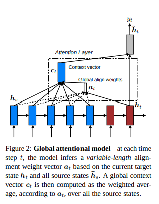
2.2 Bahdanau et al. NMT model
-
Encoder: Use RNN to process input sequence and collect \((h_1,...,h_n)\)
-
Decoder:
\[s_i=f(s_{i-1}, y_{i-1}, c_i)\]Where \(s_{i-1}\) is the previous hidden, \(y_{i-1}\) is the previous prediction, \(c_i\) is the context from the input sequence that is relevant for the current decoding job. It is calculated as follow
\(\begin{align} e_{i,j} &= a(s_{i-1}, h_j) \\ \alpha_{i,j} &= \frac{exp(e_{i,j})}{\sum_{k=1}^{n}exp(e_{i,k})} \\ c_i &=\sum_{j=1}^{n} \alpha_{i,j}h_j \\ \end{align}\) That is:
- We use the hidden state \(s_{i-1}\) to query the encoder hidden states, and create a score for each.
- Use softmax to convert these scores into a proper probability
- Finally compute the context vector as weighted average of the encoder hidden states.
- Ideally the softmax will put higher value on important stuff.
2.3 Connection with translation alignment
- The attention-based model learns to assign significance to different parts of the input for each step of the ouput.
- In the context of translation, attention can be thought of as “alignment”
- Bahdanau et al. argue that the attention scores \(\alpha_{i,j}\) at decoding step \(i\) signify the words in the input sequence that align with the word \(i\) in the output sequence.
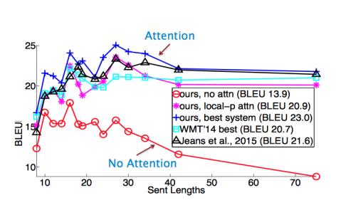
2.4 Performance on long sentence
- As the sequence length grows, models do not use attention will miss information.
17 Other NMT Models
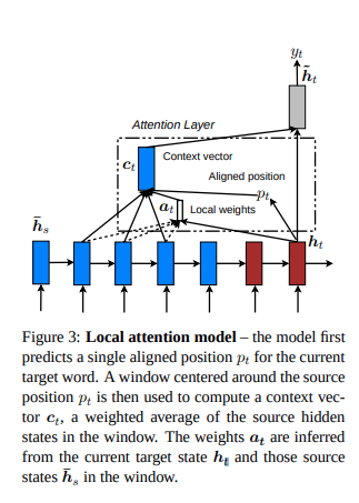
3.1 Global / Local Attention
- Many ways to do attention. Luong et al’s attention are using current hidden state to do attention and modify what to output at the current step. Sort of post activation attention, compare to Bahdanau’s pre activation attention.
- And they added some control after attention about how much around the aligned position should the information be aggregated as context.
3.2 Google’s multilingua NMT
- A Seq2Seq model that accepts as input a sequence of words and a token specifying what language to translate into.
- The model uses shared parameters to translate into any target language.
- It enabled “zero-short translation”, in which we can translate between two languages for which we have no translation training data. They can actually generate reasonable Japanese-Korean translations where they only had Japanese-English and Korean-English in training data.
- This is showing: the decoding process is not language-specific, the model is in fact maintaining an internal representation of the input / output sentences independent of the actual languages involved.
18 Sequence Model Decoders
-
Consider a model that computes the probability \(P(\bar{s} \vert s)\) of a translation \(\bar{s}\) given the original sequence \(s\). We want to pick the translation \(\bar{s}*\) that has the best probability.
\[\bar{s}*=argmax_{\bar{s}}(P(\bar{s}|s))\] -
As the search space can be huge \(\vert V \vert^{len(s)}\), we need to shrink its size:
-
Exhaustive search: compute the probability of every possible sequence, and chose the one with the highest probability. Too complex, NP_complete.
-
Ancestral sampling: at time step \(t\), we sample \(x_t\) based on the conditional probability of the word at step $t$ given the past.
\(x_t \sim P(x_t \vert x_1, \dots, x_n)\) High variance
-
Greedy search: at time step \(t\), we pick the most probable token.
\[x_t=argmax_{\tilde{x_t}}P(\tilde{x_t} \vert x1,\dots,x_n)\]Efficient, but if we make a mistake at one time step, the rest of the sentence could be heavily impacted.
-
Beam search: maintain \(K\) candidates at each time step.
\[H_t =\{(x_1^1,\dots,x_t^1),\dots,(x_1^K,\dots,x_t^K)\}\]and compute \(H_{t+1}\) by expanding \(H_{t}\) and keeping the best \(K\) candidates. In other words, we pick the best \(K\) sequence in the following set
\[\tilde{H}_{t+1} = \bigcup_{k=1}^{K}H^{\tilde{k}}_{t+1}\]where
\[H^{\tilde{K}}_{t+1} = \{(x^k_1,\dots ,x^{k}_t, v_1),\dots,(x^k_1,\dots ,x^{k}_t, v_{\vert V \vert})\}\]As we increase \(K\), we gain precision and we are asymptotically exact. Beam search is the most commonly used technique in NMT.
-
19 Evaluation of Machine Translation Systems
5.1 Human Evaluation
- Gold standard, but costly and inefficient
5.2 Evaluation against another task
- Eg. Feed translation to question answering to see if the QA model can work well with translated text.
-
Or query-retrieval task. etc
- The second task may not be affected by many of the finer points of translation.
5.3 BLEU Bilingual Evaluation Understudy
- Evaluates the precision score of a candidate machine translation against a reference human translation with n-grams matches, the score is the fraction of n-grams in the translation that also appear in the reference.
- The BLEU score has been reported to correlate well with human judgment of good translations.
20 Dealing with the large output vocabulary
- Problem: softmax can be quite expensive to compute with a large vocabulary and its complexity also scales proportionally to the vocabulary size.
6.1 Scaling softmax
-
Noise Contrastive Estimation NCE
approximate softmax by randomly sampling K words from negative samples. reduce complexity by a factor of \(\frac{\vert V \vert}{K}\)
-
Hierarchical Softmax introduce a binary tree structure to more efficiently compute softmax reduce complexity to \(log(\vert V \vert)\)
- Problem: both methods only save computation during training, when target word is known. At test time, we still has to compute the probability of all words in vocab to make predictions.
6.2 Reducing vocabulary
-
reduce vocabulary size to a small number and replace words outside the vocabulary with a tag
<UNK> -
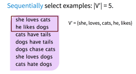
maintain a constant vocabulary size \(\vert V' \vert\) by partitioning the training data into subsets with \(\tau\) unique target words, where \(\tau = \vert V' \vert\). Very similar to NCE, that for any given word, the ouput vocabulary contains the target word and \(\vert V' \vert - 1\) negative samples. However, these negative samples are sampled from a biased distribution \(Q\) for each subset \(V'\) where:
\[Q(y_t) = \begin{cases} \frac{1}{\vert V' \vert} & if \ y_t \in \vert V' \vert \\ 0 & otherwise \end{cases}\]At test time, things are complicated.
6.3 Handling unknown words
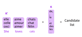
- learn to “copy” from source text (Pointer network, Gulcehre et al.)
- Applies attention distribution \(l_t\) to decide where to point in the source text and uses the decoder hidden state \(S_t\) to predict a binary variable \(Z_t\) which decides when to copy from source text.
- The final prediction is either the word \(y_t^w\) chosen by softmax over candidate list, or \(y_t^l\) copied from source text depending on the value of \(Z_t\).
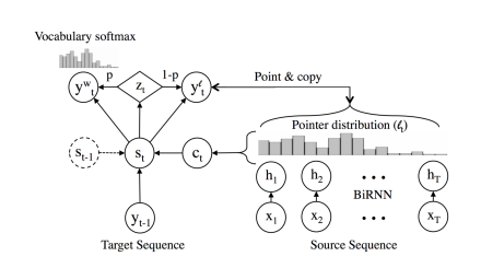
this approach is both unreliable at scale - the attention mechanism is unstable when the network is deep - and copying may not always be the best strategy for rare words - sometimes transliteration is more appropriate.
21 Word and character-based models
Another direction to address unknown words is to operate at sub-word levels
- word segmentation
- character-based
Or, to embrace hybrid architectures
7.1 Word segmentation
-
Representing rare and unknown words as a sequence of subword units.
-
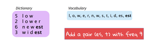
Byte Pair Encoding: start with a vocabulary of characters and keep extending the vocabulary with most frequent n-gram pairs in the data set.
- One can choose to either build separate vocabularies for training and test sets or build one vocabulary jointly.
7.2 Character-based model
-
For each word \(w\) with \(m\) characters \(c_1,c_2,\dots,c_m\) to look up the character embeddings \(e_1, e_2, \dots e_m\) These character embeddings are then fed into a biLSTM to get the final hidden states \(h_f, h_b\) . The final word embedding is computed by an affine transformation of two hidden states:
\[e_w=W_fH_f + W_bH_b + b\]
7.3 Hybrid NMT
- Translates mostly at word-level and consults the character components for rare words.
- The character-level RNN compute source word representations and recover unknown target words when needed.
- Word-based Translation as a Backbone: word-level RNN use
<UNK>for out of vocabulary words. - Source Character-based Representation: character RNN process out of vocabulary word and feed final hidden state as embedding for the word for the word-level RNN.
- Target Character-level Generation. character RNN uses word-level model’s state(which leads to
<unk>) as initial hidden and generates a word to replace<unk>
22 Self-Attention and Transformers
RNN and Attention
-
Attention in RNN: allow flexible access to memory (encoder hidden states)
-
Issues with RNNs:
-
Linear interaction distance - takes O(seq length) for distant word pairs to interact.
-
Hard to learn long-distance dependencies (gradient)
-
Linear order of words is baked in, but we know linear order isn’t the right way to think about sentences. (Tree?)
-
-
Lack of parallelizability - forward and backward passes have O(seq length) unparallelizable operations.
- Need hidden states from previous step to compute current step
- Inhibits training on very large datasets
-
Word Window and Attention
-
Word windows:
- word window models aggregate local contexts (1D convolution)
- Number of un-parallelizable operations does not increase sequence length.
- Long-distance dependencies can be captured with stacking word window layers
- Maximum interaction distance = sequence length / window size
-
Attention:
- Treats each word’s representation as a query to access and incorporate information from a set of values.
- Number of un-parallelizable opeartions does not increase sequence length.
- Maximum interaction distance: O(1), since all words interact at every layer.
-
Self-Attention:
-
queries, keys and values are drawn from the same source.
- simplest is to use v = k = q = x
-
Dot product self-attention operation is as follows:
\[\begin{align} e_{ij} = q_i^Tk_j & \qquad \text{compute key-query affinities} \\ \alpha_{ij} = \frac{exp(e_{ij})}{\sum_{j'}exp(e_{ij'})} & \qquad \text{compute attention weights from affinities (softmax)} \\ output_i = \sum_{j}\alpha_{ij}v_j & \qquad \text{compute output as weighted sum of values} \end{align}\] -
Can self-attention be a drop-in replacement for recurrence? No
- self-attention is an operation on sets. It has no inherent notion of order.
- Add position embeddings to word embeddings. Used to be hand designed sinusoidal functions, now learned as well.
- no nonlinearities for deep learning, it all just weighted averages.
- Add feed-forward network to post-process each output vector.
- Without it, stacking self-attention is just re-averages values.
- Need to ensure we don’t “look at the future” when inference.
- Mask out attention to future words by setting attention scores to \(-\infty\)
- self-attention is an operation on sets. It has no inherent notion of order.
-
Transformer (Vaswani)
-
Key-Query-Value Attention: \(k_i = Kx_i, \qquad where \ K \in \mathbb{R}^{d\times d}\\ q_i = Qx_i, \qquad where \ Q \in \mathbb{R}^{d\times d}\\ v_i = Vx_i, \qquad where \ V \in \mathbb{R}^{d\times d}\\\) These matrices allow different aspects of the \(x\) vectors to be used/emphasized in each of the three roles.
\(X = [x_1;x_2;\dots;x_T] \in \mathbb{R}^{T\times d}\) output is \(softmax(XQ(XK)^T) \times XV\)
-
Multi-Headed Attention:
What if we want to look in multiple places in the sequence for different reasons all at once?
define multiple attention heads through multiple Q,K,V matrices.
Let \(Q_l, K_l, V_l \in \mathbb{R}^{d\times \frac{d}{h}}\) where \(h\) is the number of attention heads.
Each attention head performs attention independently:
\(output_l = softmax(XQ_lK_l^Tx^T)\times XV_l\) where \(output_l \in \mathbb{R}^{d/h}\)
We then concatenate outputs to get back to the original dimension.
Each head gets to “look” at different things, and construct value vectors differently.
It is the same amount of compute as single-head attention.
-
Instead of \(X^{i} = Layer(X^{i-1})\) let \(X^{i} = X^{i-1} + Layer(X^{i-1})\)
Residual connections are thought to make the loss landscape considerably smoother -> thus easier training.
-
Cut down on uninformative variation in hidden vector values by normalizing to unit mean and standard deviation within each layer
Maybe due to its normalizing gradients
\[output = \frac{x-\mu}{\sqrt{\sigma} + \epsilon} * \gamma + \beta\]where \(\gamma\) and \(\beta\) are learned “gain” and “bias”.
-
Scaled Dot Product Attention:
When \(d\) becomes large, dot products tend to become large.
-
Multi-head Cross-Attention:
Query from Decoder and Key/Value from Encoder
- Drawbacks:
23 Subword, Transformer Pretraining
1. Word Structure and subword models
- Traditional language model assumes a fixed vocab, built from the training set, all novel words seen at test time are mapped to a single UNK token.
- Finite vocabulary assumptions make even less sense in many languages, many languages exhibit complex morphology, or word structure. E.g a single verb may have hundreds of conjugations.
- Subword modeling:
- Dominant modern paradigm is to learn a vocabulary of parts of words (subword tokens).
- At training and testing time, each word is split into a sequence of known subwords.
- The byte-pair encoding algorithm
- Start with a vocabulary containing only characters and an “end-of-word” symbol.
- Using a corpus of text, find the most common adjacent characters “a,b”; add “ab” as a subword.
- Replace instances of the character pair with the new subword; repeat until desired vocab size.
- Newer method is WordPiece.
- Common words splitted into subwords in vocab.
- Rare words splitted into subwords (sometimes intuitive, sometimes not), and in worst case, fallback to char stream.
2. Pretraining Word Embeddings
- Distributional semantics:
You shall know a word by the company it keeps - J. R. Firth
- But
the complete meaning of a word is always contextual, and no study of meaning apart from a complete context can be taken seriously - J. R. Firth
- Approach 1: Start with pretrained word embeddings only(no context, ie the same word will always get the same embedding no matter what context it is in.) and learn how to incorporate context in an LSTM or Transformer while training on the task.
- Issues:
- The downstream task may not be sufficient to teach all contextual aspects of language.
- Approach 2: All or almost all model parameters in the network are initialized via pretraining. Pretraining methods hide parts of the input from the model, and train the model to reconstruct those parts.
- This filling the blank pretraining is effective at building strong:
- representations of language
- parameter initializations for strong NLP models
- Probability distributions over language that we can sample
- Language modeling as pretraining:
- Model \(p_{\theta}(w_t \vert w_{1:t-1})\) the probability distribution over words given their past contexts.
- Pretraining model (optionally and word embedding) on language modeling task, then fine tune on the task at hand (maybe sentiment classifier).
- Stochastic gradient descent and pretrain/finetune
- Pretraining matter because SGD sticks close to the parameters \(\hat{\theta}\) from pretraining during fine tuning(if lr is small of course).
- Either:
- Fine tuning near the local minima near \(\hat{\theta}\) tend to generalize well.
- And/Or, maybe the gradients of finetuning loss near \(\hat{\theta}\) propagate nicely.
- Three pretraining schemes:
- Decoders only - Language models, nice to generate from, but can’t condition on future words
- Encoders only - Gets bidirectional context - can condition on future
- Encoder-Decoders - Good parts from above? but how do we train this
3. Decoder only pretraining
- Train decoder only language model then tune on classification / QA / summarization task.
- GPT(Radford et al. 2018) is decoder only transformer pretrained as language models.
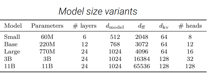
- 12 Layers of transformer decoders
- 768 - dimensional hidden states, 3072-dimensional feed-forward hidden layers
- Byte-pair encoding with 40,000 merges
- Trained on BooksCorpus: over 7000 unique books
- GPT = Generative PreTraining / Generative Pretrained Transformer
- GPT decoder finetuning task:
- Natural Language Inference - label pairs of sentences as entailing / contradictory / neutral
- [START] The man is in the doorway [DELIM] The person is near the door [EXTRACT]
- The linear classifier is applied to the representation of the [EXTRACT] token.
- The next generation GPT2 showed better natural language generations.
4. Encoder only pretraining
-
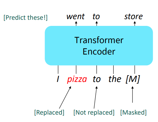
Since encoders get bidirectional context, we can’t do language modeling. Instead we predict masked words. Called Masked LM.
-
Only add loss terms from words that are “masked out”. Learn \(p_{\theta}(x \vert \tilde{x})\) where \(\tilde{x}\) is the masked version of the sequence.
- BERT (Devlin et al, 2018) is encoder only transformer pretrained on masked language model objective.
- Predict a random 15% of (sub)word tokens.
- Replace input word with [MASK] 80% of the time
- Replace input word with a random token 10% of the time
- Leave input word unchanged 10% of the time (but still predict it)
- Why? Doesn’t let the model get complacent and not build strong representations of non-masked words.
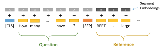
- The pretraining input to BERT was two separate contiguous chunks of text:
[CLS] my dog is cute [SEP] he likes play ##ing [SEP] A A A A A A B B B B B 0 1 2 3 4 5 6 7 8 9 10- Two released model:
- base - 12 layers, 768-dim hidden states, 12 attention heads, 110 million params
- large - 24 layers, 1024-dim hidden states, 16 attention heads, 340 million params
- Trained on Books Corpus + English wikipedia
- Trained on 64 TPU chips
- Fine tuning is practical and common on a single GPU
- Predict a random 15% of (sub)word tokens.
-
Limitations of pretrained encoders
- pretrained encoders don’ naturally lead to nice autoregressive (1-word-at-a-time) generation methods.
-
BERT extensions: like RoBERTa, SpanBERT, etc
- RoBERTa: train BERT for longer and remove next sentence prediction! More compute, more data can improve pretraining even when not changing the underlying transformer encoder.
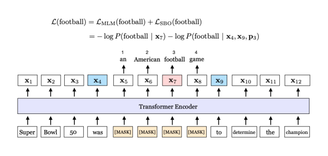
- SpanBERT: masking contiguous spans of words makes a harder, more useful pretraining task
5. Encoder-Decoder pretraining
- Encoder portion can benefits from bidirectional context; and the decoder portion is used to train the whole model through language modeling.
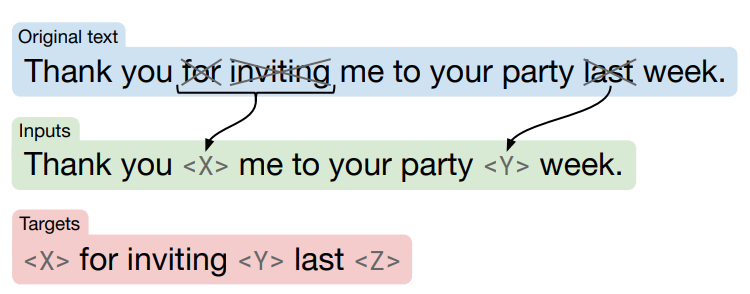
- Objective: Span corruption(denoising). T5 (Raffel et al, 2018)
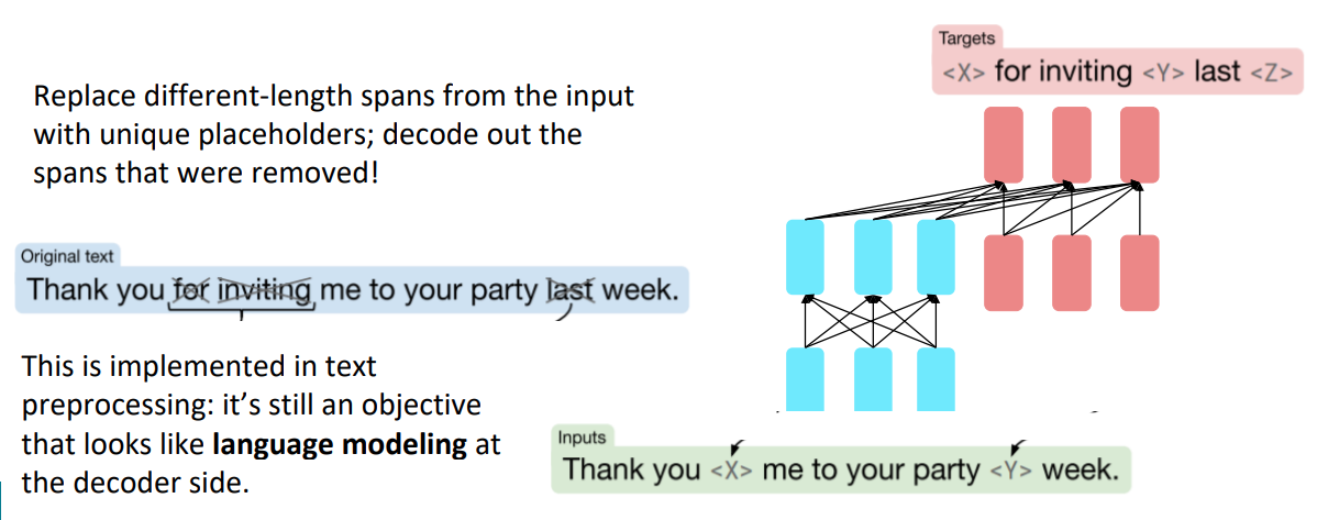
- They found encoder-decoder work better than decoders only, and span corruption work better than language modeling.
- T5 was tuned on wide range of QA tasks, NQ(Natural Questions), WQ(WebQuestions), TQA(Trivia QA).
6. What do we think pretraining is teaching?
- There is increasing evidence that pretrained models learn a wide variety of things about the statistical properties of language.
- Stanford University is located in __, California. [Trivia]
- I put _ fork down on the table. [syntax]
- The woman walked across the street, checking for traffic over _ shoulder. [coreference]
- I went to the ocean to see the fish, turtles, seals, and _____. [lexical semantics/topic]
- Overall, the value I got from the two hours watching it was the sum total of the popcorn and the drink. The movie was _. [sentiment]
- Iroh went into the kitchen to make some tea. Standing next to Iroh, Zuko pondered his destiny. Zuko left the . [some reasoning – this is harder]
- I was thinking about the sequence that goes 1, 1, 2, 3, 5, 8, 13, 21, [some basic arithmetic; they don’t learn the Fibonnaci sequence]
- Models also learn – and can exacerbate racism, sexism, all manner of bad biases.
7. Very Large Models
- Two ways of interact with pretrained models:
- Sample from the distributions they define(maybe providing a prompt)
- Fine-tune them on a task we care about, and take their predictions
- Very large language models seem to perform some kind o f learning without gradient steps simply from examples you provide within their contexts.
- GPT-3 is the canonical example of this, 175 billion parameters. (T5 is 11 billion)
- The in-context examples seem to specify the task to be performed, and the conditional distribution mocks performing the task to a certain extent.
- input: “thanks->merci; hello->bonjour; mint->menthe; otter -> “ output “loutre”
24 Question Answering
Overview
-
What is question answering?
- build systems that automatically answer questions posed by humans in a natural language
- Question types
- Factoid vs non-factoid, open-domain vs closed domain, simple vs compositional
- Answer types
- short segment of text, a paragraph, a list, yes/no, …
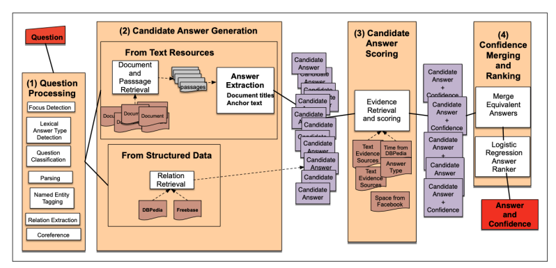
- IBM Watson
- Deep learning era: all SOTA QA systems are built on top of end-to-end training and pre-trained language models.
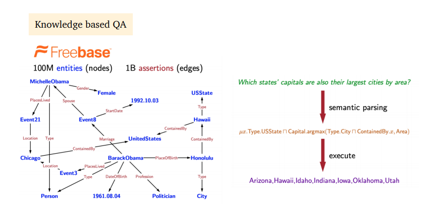
- There are also QA system built with knowledge graphs.
Reading Comprehension
- comprehend a passage of text and answer questions about its content \((P, Q) \rightarrow A\)
- many other NLP tasks can be reduced to a reading comprehension problem:
- Information extraction:
- Barack Obama, educated_at, ? -> where did Barack Obama graduate from?
- Semantic role labeling
- etc
- Information extraction:
- SQuAD(Stanford question answering dataset)
- 100k annotated (Passage, Question, Answer) triples
- Passages are from English Wikipedia, usually 100~150 words
- Questions are crowd-sourced
- Each answer is a span in the passage - not all questions can be answered in this way. 3 gold answers per questions
- Evaluation is exact match(0/1) or F1
- Human reference: EM 82.3% F1 91.2
- Problem formulation:
- Input: \(C=(c_1, c_2, \dots, c_N), Q=(q_1, q_2, \dots, q_n)\)
- Output: \(1 \leq start \leq end \leq N\)
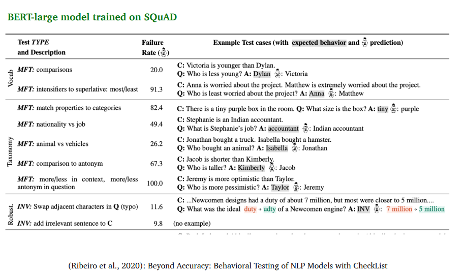
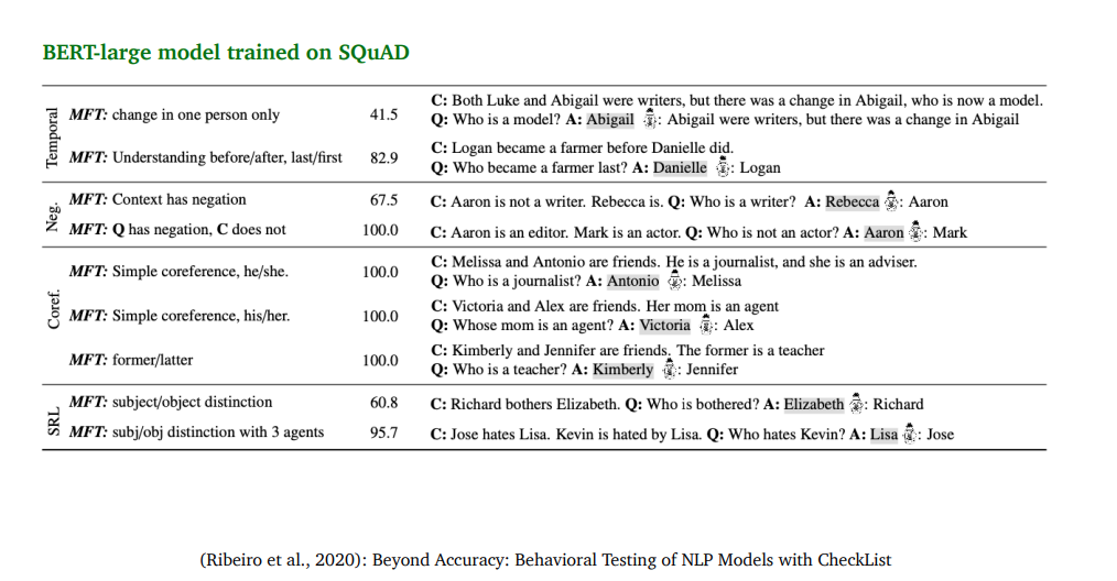
- 2016-2018: A family of LSTM-based models with attention
- 2019+: Fine-tuning BERT-like models
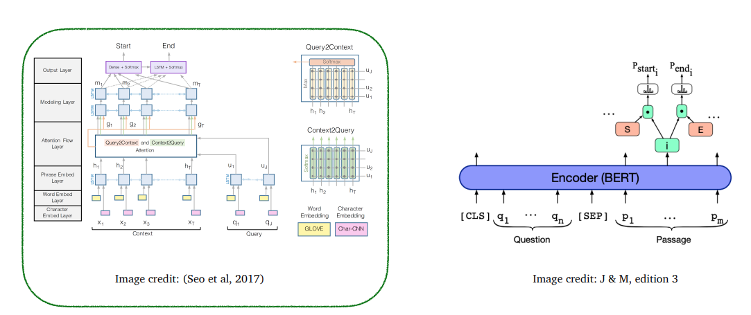
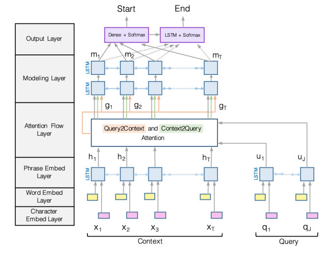
BiDAF: the Bidirectional Attention Flow model
-
Encoding:
-
Use a concatenation of word embedding (GloVe) and character embedding (CNNs over character embeddings) for each word in context and query
\[e(c_i) = f([GloVe(c_i);charEmb(c_i)])\]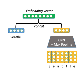
-
Then use two bidirectional LSTMs separately to produce contextual embeddings for both context and query
-
-
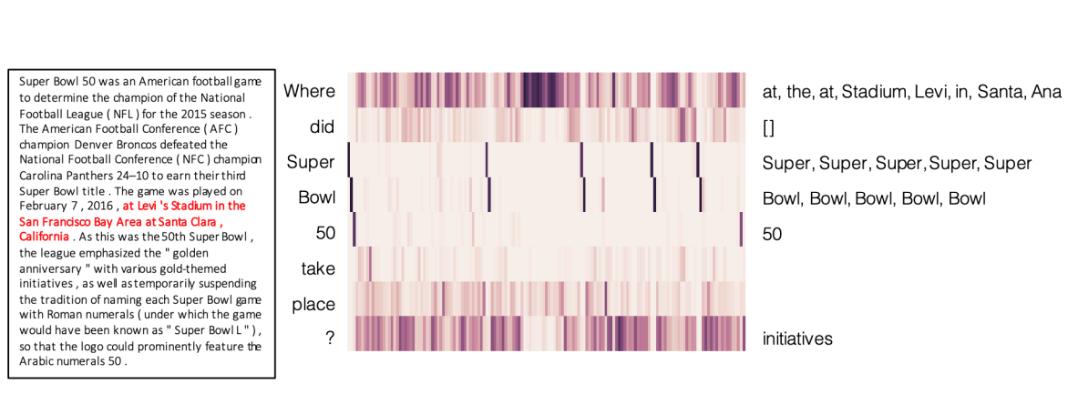
Attention:
-
Context-to-query attention: for each context word, choose the most relevant words from the query words
-
Query-to-context attention: choose the context words that are most relevant to one of the query words
-
Compute:
-
First, similarity score for every pair of \((c_i, q_j)\):
\[S_{i,j} = w^T_{sim}[c_i;q_j;c_i\odot q_j] \in \mathbb{R} \qquad w_{sim} \in \mathbb{R}^{6H}\] -
Context-to-query attention (which question words are more relevant to \(c_i\)):
\[\alpha_{i,j} = softmax_j(S_{i,j}) \in \mathbb{R} \qquad a_i = \sum_{j=1}^{M}\alpha_{i,j}q_j\in \mathbb{R}^{2H}\] -
Query-to-context attention (which context words are relevant to some question words):
\[\beta_{i} = softmax_i(max_{j=1}^{M}(S_{ij})) \in \mathbb{R}^N \qquad b=\sum_{i=1}^{N}\beta_{i}c_{i} \in \mathbb{R}^{2H}\]
-
-
The final output is:
\[g_i = [c_i;a_i;c_i\odot a_i;c_i\odot b] \in \mathbb{R}^{8H}\]
-
-
Modeling Layer:
-
pass \(g_i\) to another two layers of bi-directional LSTMs
-
Attention layer is modeling interactions between query and context
-
Modeling layer is modeling interactions within context words(annotated with query?)
\[m_i = BiLSTM(g_i)\in \mathbb{R}^{2H}\]
-
-
Output Layer:
-
two classifier
-
s predicting the start and end position:
\[p_{start} = softmax(w^T_{start}[g_i;m_i]) \\ p_{end} = softmax(w^T_{end}[g_i;m'_i]) \\ m'_i = BiLSTM(m_i) \in \mathbb{R}^{2H} \\ w_{start}, w_{end} \in \mathbb{R}^{10H}\]
-
-
Performance:
- 77.3 F1 on SQuAD v1.1
- 67.7 F1 without context-to-query attention
- 73.7 F1 without query-to-context attention
- 75.4 F1 without character embeddings
BERT for reading comprehension
- Question = Segment A
- Passage = Segment B
- Answer = predicting two endpoints in segment B
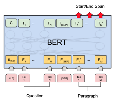
- Performance: beat human reference
Compare BiDAF and BERT
- BERT is 100 times larger than BiDAF in terms of #parameters
- BiDAF is attention connected multiple LSTM models, whereas BERT is Transformer.
- But, fundamentally they are not much different:
- BiDAF models attention of (P,Q) and (Q, P)
- BERT models attention of (P,Q), (Q, P) and (Q, Q) and (P, P) on top of BiDAF, through its self attention.
- Can we design better pre-training objectives for BERT for QA? - SpanBERT (Joshi & Chen et al, 2020)
- Masking contiguous span of words instead of random masking
- using two end points of span to predict all the masked words in between = compressing the information of a span into its two endpoints.
Is reading comprehension solved? No
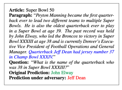
-
Even though BERT already out-performed human on SQuAD, but the systems still perform pooly on adversarial examples or examples from out-of domain distributions.
-
Also, systems trained on one dataset can’t generalize to other datasets.
Open-domain question answering
-
Different from reading comprehension, we don’t assume a given passage
-
Only have access to a large collection of documents, we don’t know where the answer is located.
-
Retriever-reader framework (eg. Dr.QA)
- Input: a large collection of documents \(\mathit{D}=D_1, D_2, \dots, D_N$ and $Q\)
- Output: an answer string $A$
- Retriever: \(f(D, Q) \rightarrow P_1, \dots, P_K\) K is pre-defined (e.g. 100)
- Reader: \(g(Q, {P_1, \dots, P_K}) \rightarrow A\) A is a reading comprehension problem
-
In Dr.QA:
- Retriever = A standard TF-IDF information-retrieval sparse model ( a fixed module)
- Reader = a neural reading comprehension model
-
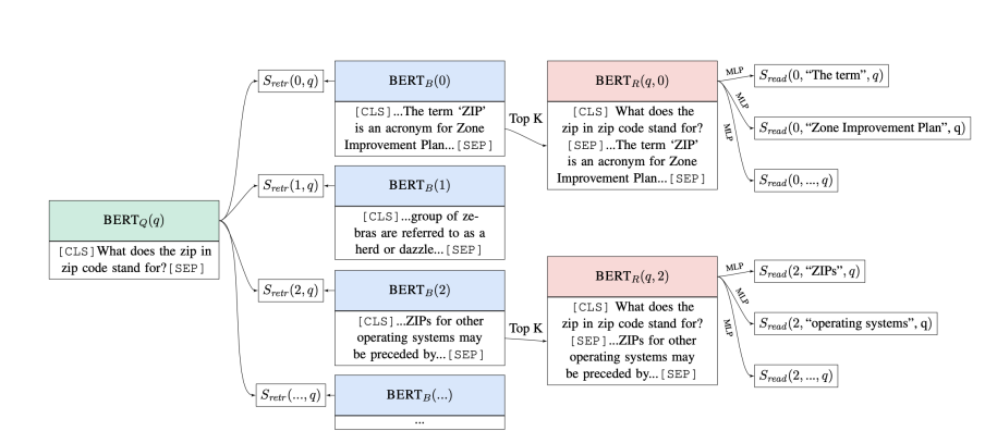
Latent Retrieval for Weakly Supervised Open Domain Question Answering (Lee, et al, 2019)
- Joint training of retriever and reader
- Each text passage can be encoded as a vector using BERT and the retriever score can be measured as the dot product between the question representation and passage representation
- However, it is not easy to model as there are huge number of passages
-
Dense Passage Retrieval for Open-Domain Question Answering (Karpukhin et al. 2020)
- DPR - train the retriever using question-answer pairs
- Trainable retriever largely outperforms traditional IR retrieval models. (1K pairs beats BM25)
-
Leveraging Passage Retrieval with Generative Models for Open Domain Question Answering
- Recent work shows that it is beneficial to generate answers instead of to extract answers
- Fusion-in-decoder (FID) = DPR + T5
-
How Much Knowledge Can You Pack Into the Parameters of a Language Model? (Roberts et al, 2020)
- Large Language models can do open-domain QA well
- without an explicit retriever stage
- Tuning T5
-
Real-Time Open-Domain Question Answering with Dense-Sparse Phrase Index (Seo et al, 2019)
-
Learning Dense Representations of Phrases at Scale (Lee, et al, 2020)
- It is possible to encode all the phrases using dense vectors and only do nearest neighbor search without a BERT model at inference time
25
- Examples of NLG:
- Machine Translation
- Dialogue Systems
- Summarization
- Data-to-Text Generation
- Visual Description
- Creative Generation
-
NLG: any task involving text production for human consumption.
- Basics of NLG
- Autoregressive model: predict \(\hat{y}_t = f(\{y_{<t}\})\)
- Score \(S \in \mathbb{R}^{\vert V \vert} = f(\{y_{<t}\})\)
- Distribution \(P\) over \(w \in V\): \(P(y_t=w \vert \{y_{<t}\})=\frac{exp(S_w)}{\sum_{w'\in W}exp(S_{w'})}\)
- Training: minimizing \(L_t = -logP(y_t \vert \{y_{<t}\})\)
- Inference: \(\hat{y}_t=g(P(y_t \vert \{y_{<t}\}))\) where \(g\) is the decoding algorithm
- Decoding algorithms
- Greedy methods:
- argmax decoding: \(\hat{y}_t = \underset{w\in W}{argmax}P(y_t=w \vert y_{y<t})\)
- Beam Search:
- Greedy methods heavily focus on high probable sequence, not random enough to match human.
- Overall, maximum probability decoding is good for low-entropy tasks like MT and summarization.
- Dealing with repetition:
- Heuristic: Don’t repeat n-grams
- Complex:
- Minimize embedding distance between consecutive sentences: does not help with intra-sentence repetition
- Coverage loss: prevents attention from attending to the same words
- Unlikelihood objective: Penalize generation of already-seen tokens
- Use a different decoding objective: Contrastive decoding searches for strings x that maximize \(logprob_{largeLM}(x) - logprob_{smallLM}(x)\)
- Top-k sampling:
- Sample from the top k tokens in the probability distribution
- Increase k for more diverse / risky outputs
- Decrease k for more generic / safe outputs
- Problem:
- The distributions we are sample from are dynamic
- When P is flat, limited k removes many viable options
- When P is peakier, a high k allows for too many options
- Top-p (nucleus) sampling:
- Sample from all tokens in the top p cumulative probability mass
- Varies k depending on the uniformity of P
- Newer sampling methods:
- Typical Sampling: Reweights the score based on the entropy of the distribution.
- Epsilon Sampling: Set a threshold for lower bounding valid probabilities.
- Scaling randomness:
- Softmax temperature \(P_t(y_t=w) = \frac{exp(S_w/\tau)}{\sum_{w' \in V}exp(S_{w'}/\tau)}\)
- Raise the temperature \(\tau > 1\): \(P\) becomes more uniform -> more diverse output
- Lower the temperature \(\tau < 1\): \(P\) becomes more spiky -> less diverse output
- temperature is hyper-parameter for decoding methods
- Re-balancing distributions
- Re-balance \(P\) using retrieval from n-gram phrase statistics
- Back propagation-based distribution re-balancing:
- Latent –foward–> sentiment scoring model
- Latent <-backward- loss
- Latent –decoder–> P
- Re-ranking
- Generate a bunch sequences, use one or more re-rankers to score / rank them and pick one
- Different decoding algorithms can allow us to inject biases that encourage different properties of the generated text.
- Self-consistency decoding
- Greedy methods:
- Training NLG models
- Exposure Bias
- Training with teacher forcing leads to exposure bias at generation time.
- Solutions:
- Scheduled sampling - sometimes use a decoded token as next input rather than golden token during the training.
- Dataset Aggregation - gradually mixin model’s predicted sequences into training set.
- Retrieval Augmentation - learn to retrieve a sequence from corpus and edit it to match desired output.
- Reinforcement Learning - Many rewards choices - RLHF is latest
- Exposure Bias
26 Coreference Resolution
What is Coreference Resolution?
-
Identify all mentions that refer to the same entity in the word
- Step 1: Detect the mentions
- Step 2: Cluster the mentions
-
Mention Detection: A span of text referring to some entity
- Pronouns
- Named entities
- Noun phrases
-
Keep all mentions as candidates, running them through coreference system and discard singleton mentions.
-
Or we can train end-to-end model
-
Four kinds of coreference models:
- Rule-based (pronominal anaphora resolution)
- Hobbs’ naive algorithm 1976
- Knowledge-based 0 Winograd Schema
- Mention Pair (binary classification)
- Mention Ranking (softmax)
- Clustering
- Rule-based (pronominal anaphora resolution)
-
Non-Neural Coref Model: Features
- Person / Number / Gender agreement
- Semantic compatibility
- Certain syntactic constraints
- More recently mentioned entities preferred for referenced
- Grammatical Role: Prefer entities in the subject position
- Parallelism
-
Neural Coref Model
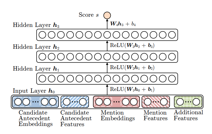
- Embeddings:
- previous two words, first word, last word, head word etc of each mention
- distance, document genre, speaker information etc
- Embeddings:
Convolutional Neural Nets
-
1d discrete convolution definition:
\[(f*g)[n] = \sum_{m=-M}^Mf[n-m]g[m]\] - Convolution is classically used to extract features from images
-
batch_size = 16 word_embed_size = 4 seq_len = 7 x = torch.randn(batch_size, word_embed_size, seq_len) conv1 = Conv1d(in_channels=word_embed_size, out_channels=3, kernel_size=3, padding=1) hidden1 = conv1(x) hidden2 = torch.max(hidden1, dim=2) # max pooling- Models position-invariant identification
- filter is of size: kernel_size x in_channels
- number of filters is the same as number of desired output channels
- output seq len depends on padding, kernel size and seq_len as well as stride
End-to-end Model
- Embed words in the document using a word embedding matrix and a character-level CNN
- Then run a bidirectional LSTM over the document
- Next, represent each span of text i going from start(i) to end(i) as a vector
- Span representation: \(g_i=[x^*_{start(i)},x^*_{end(i)},\hat{x_i},\phi(i)]\)
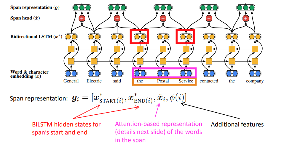
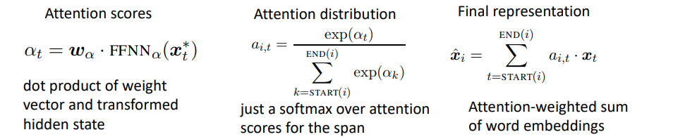
- \(x^*_{start(i)}\) gives the context to the left
- \(x^*_{end(i)}\) gives the context to the right
- \(\hat{x_i}\) gives the representation of the span
-
\(\phi(i)\) gives other information in the text
-
Lastly score every pair of spans:
\[s(i, j) = s_m(i) + s_m(j) + s_a(i,j) \\ s_m(i) = w_m \cdot FFNN_m(g_i) \\ s_a(i, j) = w_a \cdot FFNN_a([g_i, g_j, g_i \odot g_j, \phi(i, j)])\] -
Intractable to score every pair of spans
- \(O(T^2)\) spans of text in a document
- \(O(T^4)\) runtime
- Lots of pruning to work on
- Attention learns which words are important in a mention (like head words)
BERT-based coref:
- SpanBERT: pretrains BERT models to be better at span-based prediction tasks like coref and QA
- BERT-QA for coref: Treat Coreference like a deep QA task:
- Point to a mention, and ask “what is its antecedent”?
- Answer span is a coreference link
Coreference Evaluation
- Many different metrics: MUC, CEAF, LEA, B-CUBED, BLANC, F1 score average over 3 coreference metrics
- Dataset: OntoNotes dataset ~ 3000 documents labeled by humans
27 T5 and Large Language Models
Which transfer learning methods work best and what happens when we scale them up?
-
T5 - Text-to-Text Transfer Transformer
-
Downstream tasks
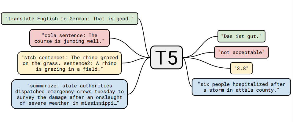
-
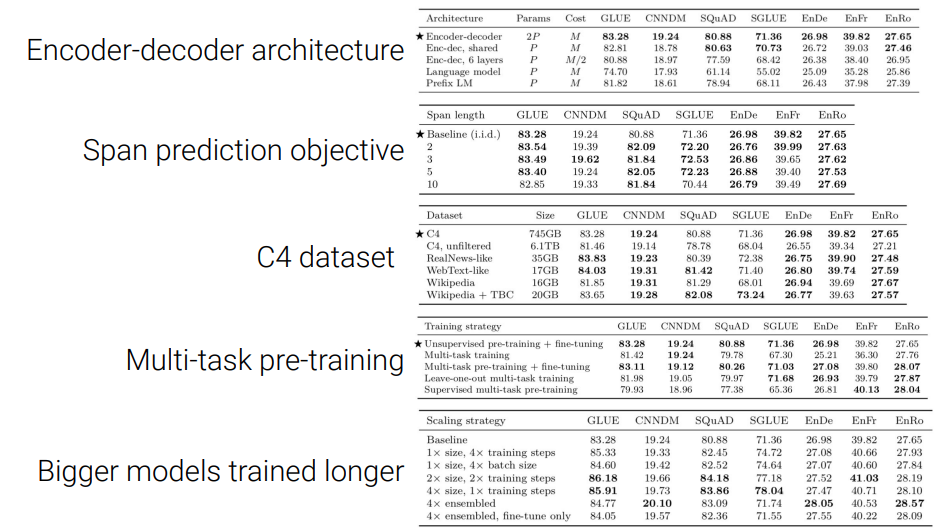
Architecture: standard BERT
-
Dataset: C4 (processed common crawl)
-
Pretraining task: Span prediction (Denoising objective)
- Multitask learning, how often I sample from each task? Often hurt single task performance compare to tune single task. Each task has its own prefix(like “stsb”, “summarize” etc)
- Best-strategy: Multitask learning with task data + unsupervised pretraining data -> fine tuning on single tasks
- Scale:
- larger model train longer > even larger model > training even longer > ensemble!
How much knowledge does a language model pick up during pre-training?
-
pretrained T5 LM tested on closed-book QA(no retrieval)
-
Gap behind SOTA systems, but larger model score better -> suggests larger model pick up more knowledge?
-
Add Salient Span Masking - REALM: Retrieval-Augmented Language Model Pre-Training (Guu et al)
- Mask entire entity
Greatly improved QA close to SOTA
Domain/Task Adaptive pretraining
-
How do we know when language model know? - highly calibrated model will not produce high confident score for the predictions when it does not know the answer.
-
Fun fact: T5 peaked downstream task performance before a single pass on the tuning set. -> unlikely the model overfits the down stream task data.
Do large language models memorize their training data?
-
GPT2 has memorized its training data. Prefix East Stroudsburg Stroudsburg->
-
Larger model memorize more data, even when the data only occur very rarely…
Can we close the gap between large and small models by improving the Transformer archtecture?
- Modifications:
- Factorized embedding
- Shared embedding and softmax layer
- Mixture of Softmaxes / adaptive Softmax
- Different way of initializing / normalizing the model
- Different attention mechanism
- Different structure for the feed forward network: mixture of experts, switch transformer, different nonlinearities.
- Funnel Transformer, Evolved Transformer, Universal Transformer, block sharing.
- Nothing work obviously better. Nothing statistically significant
Reference
- https://arxiv.org/abs/1910.10683
- https://arxiv.org/abs/2010.11934
- https://arxiv.org/abs/2002.08910
- https://arxiv.org/abs/2012.07805
- https://arxiv.org/abs/2102.11972
28 Integrating Knowledge in Language Model
Recap Language Models
- Standard is to predict next word; recently the masked language models predict masked tokens
- Used to do language generation or evaluating the probability of text:
- summarization
- dialogue
- autocompletion
- machine translation
- fluency evaluation
- Can a language model be used as a knowledge base? (Petroni et al. 2019)
- predictions generally make sense (e.g. the correct types), but are not all factually correct
- maybe due to:
- unseen facts: fact not in training corpora
- rare facts: hasn’t seen enough examples to memorize the fact
- model sensitivity: e.g. can answer ‘x was made in y’, but not ‘x was created by y’
- Unable to reliably recall knowledge
- Knowledge-aware language models
- LM can benefit downstream tasks that leverage knowledge
- e.g. entity relation extraction
- Can language model replace knowledge base?
- Pro:
- LM trained on unlabeled data; KB is manual annotated or complex NLP pipelines
- LM support more flexible natural language queries; KB query by triplets
- Cons:
- LM is hard to interpret, why it says so?
- LM is hard to trust, incorrect answer instead of can deduce answer from KB
- LM is hard to modify, thinking about retrain to fix a single error?
- Pro:
- LM can benefit downstream tasks that leverage knowledge
Techniques to add knowledge to LMs
-
Categories
- Add pretrained entity embeddings
- ERNIE
- KnowBERT
- Use a external memory
- KGLM
- KNN-LM
- Modify the training data
- WKLM
- ERNIE, - salient span masking
- Add pretrained entity embeddings
-
1 Add pretrained entitiy embeddings
-
USA, US, United States will have different word embeddings, but should have same entity embedding. If we can correctly link the word token of entity to its entity id. We can incorporate pretrained entitiy embeddings trained via:
- Knowledge graph embedding methods - TransE
- Word-entity co-occurrence methods - Wikipedia2Vec
- Transformer encodings of entity descriptions - BLINK
-
How do we incorporate pretrained entitiy embeddings from a different embedding space?
-
Learn a fusion layer to combine context and entity information
\(h_j = F(W_tw_j + W_ee_k + b)\) where \(w_j\) is the word embedding and \(e_k\) is the entity embedding
-
-
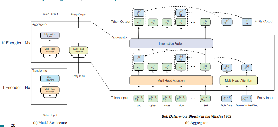
ERNIE: Enhanced Language Representation with Informative Entities (Zhang et al. ACL 2019)
-
Text encoder: BERT like
-
Knowledge encoder: stacked blocks composed of:
-
Two multi-headed attentions (MHAs) over entity embeddings and token embeddings
-
A fusion layer to combine the output of the MHAs
-
Trained with BERT objective + a knowledge pretraining task (dEA - denoising entity autoencoder, Vincent et al. ICML 2008): randomly mask token-entity alignments and predict the corresponding entity for a token from the entities in the sequence.
-
-
Remaining challenges:
- Needs text data with entities annotated in the input.
-
-
KnowBERT: Jointly learn to link entities with KnowBERT (Peters et al. EMNLP 2019)
- pretrain an integrated entity linker (EL) as an extension to BERT
- EL predicts entities so entity annotations aren’t required
- Learning EL may better encode knowledge
- Also uses a fusion layer to combine entity and context information and adds a knowledge pretraining task.
-
-
2 Use an external memory
-
Are their more direct ways than pretrained entity embeddings to provide the model factual knowledge?
-
Yes: Give the model access to an external memory (a key-value store with access to KG triplets or context information)
-
Advantages:
- Can better support injecting and updating factual knowledge
- More interpretable
-
Knowledge-Graphs for Fact-Aware Language Modeling (Logan et al. ACL 2019)
- Key idea: condition the language model on a knowledge graph
\(P(x^{t+1}, \epsilon^{t+1} \vert x^{t-m}, \epsilon^{t-m},\dots,x^{t}, \epsilon^{t})\) where \(\epsilon^{t}\) is the KG entities mentioned at timestep \(t\)
- Build a “local” knowledge graph as you iterate over the sequence
- Local KG: subset of the full KG with only entities relevant to the sequence
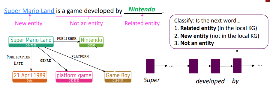
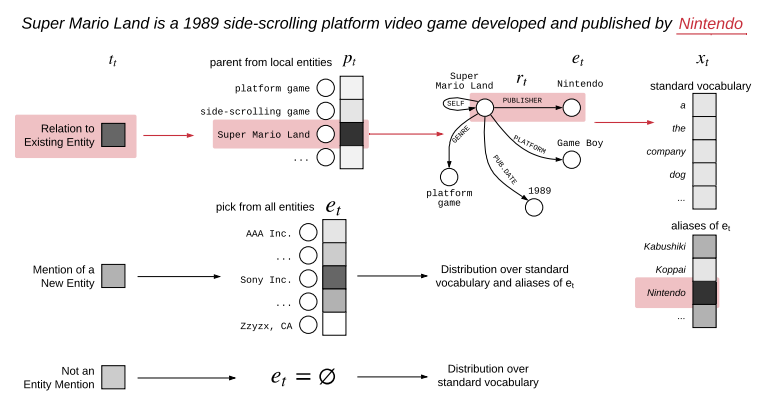
- LSTM hidden state used to predict the types of the next word:
- Related Entity (in the local KG)
- Find the top-scoring parent and relation in the local KG using the LSTM hidden state and pretrained entity and relation embeddings
- \(P(p_t) = softmax(v_p \cdot h_t)\), where \(p_t\) is the “parent” entity, \(v_p\) is the corresponding entity embedding, and \(h_t\) is from the LSTM hidden state
- Next entity: tail entity from KG triple of (top parent entity, top relation, tail entity)
- Next word: most likely next token over vocabulary expanded to include entity aliases.
- New entity ( not in the local KG)
- Find the top-scoring entity in the full KG using the LSTM hidden state and pretrained entity embeddings
- Next entity: directly predict top-scoring entity
- Next word: most likely next token over vocabulary expanded to include entity aliases
- Not an entity
- Next entity: None
- Next word: most likely next token over standard vocabulary
- Related Entity (in the local KG)
-
KGLM outperforms GPT-2 and AWD-LSTM on a fact completion task
-
Qualitatively, compared to GPT-2, KGLM tends to predict more specific tokens
-
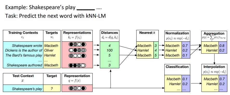
Nearest Neighbor Language Models (KNN-LM) (Khandelwal et al ICLR 2020)
-
Key idea: learning similarities between text sequences is easier than predicting the next word
-
Example: “Dickens is the author of _” \(\approx\) “Dickens wrote _”
-
Qualitatively, researchers find this especially true for “long-tail patterns”, such as rare facts
-
So, store all representations of text sequences in a nearest neighbor datastore
-
At inference:
-
Find the k most similar sequences of text in the datastore
-
Retrieve the corresponding values (i.e. the next word) for the k sequences
-
Combine the KNN probabilities and LM probabilities for the final prediction
\[P(y\vert x) = \lambda P_{KNN}(y\vert x) + (1-\lambda)P_{LM}(y\vert x)\]
-
-
-
3 Modify the training data
-
Question: Can knowledge also be incorporated implicitiy through the unstructured text?
-
Answer: Yes! Mask or corrupt the data to introduce additional training tasks that require factual knowledge.
-
Advantages:
- No additional memory / computation requirements
- No modification of the architecture required
-
Pretrained Encyclopedia: Weakly Supervised Knowledge Pretrained Language Model(WKLM) (Xiong et al. ICLR 2020)
- Key idea: train the model to distinguish between true and false knowledge
- Replace mentions in the text with mentions that refer to different entities of the same type to create negative knowledge statements (Swap noise???)
- Model predicts if entity as been replaced or not
- Type-constraint is intended to enforce linguistically correct sentences
- eg.
- True knowledge statement: J.K. Rowling is the author of Harry Potter
- Negative knowledge statement: J.R.R Tolkien is the author of Harry Potter
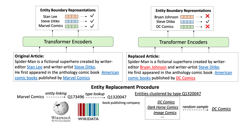
-
Uses an entity replacement loss to train the model to distinguish between true and false mentions
\[L_{entRep} = \prod_{e\in\epsilon^{+}}logP(e\vert C) + (1- \prod_{e\in\epsilon^{+}})log(1-P(e\vert C))\] -
Total loss is the combination of standard masked language model loss and the entity replacement loss
\[L_{WKLM} = L_{MLM} + L_{entRep}\] -
MLM is defined at the token level, entRep is defined at the entity level.
-
ERNIE: Enhanced Representation through Knowledge Integration
- Learn inductive biases through masking
- Can we encourage the LM to learn factual knowledge by being clever about masking?
- phrase level and entity level masking
- salient span masking to mask out salient spans (named entities and dates)
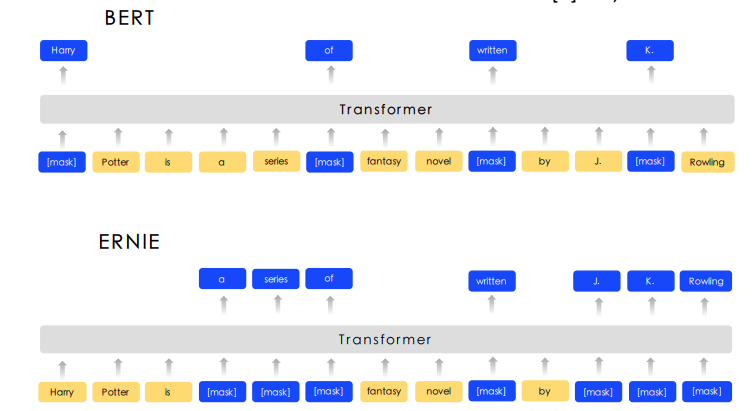
-
Recap: Techniques to add knowledge to LMS
- Use pretrained entity embeddings
- Often too difficult to apply to existing archtectures to leverage KG pretraining
- Indirect way of incorporating knowledge and can be hard to interpret
- Add an external memory
- Can support some updating of factual knowledge and easier to interpret
- Tend to be more complex in implementation and require more memory
- Modify the training data
- Requires no model changes or additional computation. May also be easiest to theoretically analyze! Active area of research
- Still open question if this is always as effective as model changes
Evaluating knowledge in LMs
-
Probe or Downstream tasks like QA
- LAnguage Model Analysis (LAMA) Probe
- How much relational (commonsense and factual) knowledge is already in off-the-shelf language models? - without any additional training or fine-tuning
- Manually constructed a set of cloze statements to assess a model’s ability to predict a missing token:
- The theory of relativity was developed by [MASK].
- The native language of Mammootty is [MASK].
- Ravens can [MASK].
- You are likely to find a overflow in a [MASK].
- Developing better prompts to query knowledge in LMs (Jiang et al TACL 2020)
- LMs may know the fact but failed on completion tasks like LAMA due to the query itself.
- the fact in pretraining data may have different contexts and sentence structure than the query.
- eg: The birth place of Barack Obama is Honolulu, Hawaii. vs Barack Obama was born in ___
- Generate more LAMA prompts by mining templates from Wikipedia and generating paraphrased prompts by using back-translation
- Ensemble prompts to increase diversity of contexts that fact can be seen in.
- LMs may know the fact but failed on completion tasks like LAMA due to the query itself.
- Can we learn a prompt???
29 Model Analysis and Explanation
Motivating model analysis and explanation
- why do model predict what it predict?’
- understanding how far we can get incremental improvements on current methods is crucial to the eventual development of major improvements
One model at multiple levels of abstraction
-
At what level of abstraction you want to reason about your model?
-
Model is a probability distribution and decision function
-
Model is a sequence of vector representations in depth and time
-
parameter weights, specific mechanisms like attention, dropout, etc
-
Out-of-domain evaluation sets
Influence studies and adversarial examples
Analyzing representations
Revisiting model ablations as analysis
30 Representing and Using Knowledge in NLP - with a focus on memory-augmented models
Topics
- How do language models currently represent knowledge?
- What makes a good knowledge representation?
- How can we build better representations? (memory-augmented models)
How do language models represent knowledge?
The part of the intestine most commonly affected by Crohn’s disease is ___
GPT-2: the rectum Correct answer: the ileum
This incorrect belief is stored somewhere in the model’s parameters. But where?
- Token embeddings?
- Feedforward layers?
- Attention layers?
Recent research on knowldge editing
- LM’s original belief: Eiffel Tower is located in the city of ___ -> Paris
- Desired edit: Eiffel Tower is located in the city of ___ -> Rome
- Model should understand full implications of edit: The tallest structure in Rome is ___ -> Effiel Tower
When and where does the model recall knowledge about the Eiffel Tower?
Causal probing:
- Add random noise to word embeddings for “Eiffel Tower” -> breaks the model
- Try to restore each layer to its original value
- See which layer is best at restoring original prediction
-> Meng et al found that FF layers above the last token of “Eiffel Tower” matter the most.
Modifying the memory -> modify columns of W_2 to change model’s behavior
- Subtract word vector for Paris, add word vector for Rome? (Dai et al. 2021)
- apply a rank-1 update: \(W_2 = W_2 + UV^T\) ~Maximize probability of outputting Rome when we see “Eiffel Tower” selector.
- Minimize change in behavior of W_2 on other inputs.
Main takeaways:
- Transformer feedforward networks can be viewed as key-value memories
- Transformers tend to look up information about an entity on the last token where it’s mentioned
- Conclusions may change as this is new research area.
What makes a good knowledge representation?
What is missingh from Transformers right now?
- We can automatically acquire knowledge from the web, but
- a lot of it is noisy or incorrect: misinformation, rumors, opinions
- we cannot trace the model’s knowledge back to an attributable source
- We can edit individual facts inside a Transformer’s memory, but
- it doesn’t work reliably yet
- current approaches break down after multiple edits
- We can store knowledge inside feedforward layers, but
- current memory capacity is too small, and scaling up is expensive
Wishlist:
- Fast and modular knowledge editing
- Robustly update the model N times without breaking its behavior on other tasks
- Attribution and interpretability
- Trace a model’s knowledge back to a particular document / training example
- Efficient scaling
- Increase the model’s memory size by 10x without paying 10x more compute
31 Memory-augmented models
A memory could be:
- Document on the web
- Record in a database
- Training example
- Entity embedding
Potentially meets our wishlist
[Input] ----------------> [NN model]------>[Output]
   |                         ^
   V                         |
[Memory Retriever]           |
   |                         |
   V                         |
[Knowledge Base] -------> [Memory]
What are some applications?
- Open-domain dialog / question answering -> Retrieve documents on the web
- Code generation -> Retrieve code snippets from Stack Overflow
- Image generation -> Retrieve reference pictures of people, places, etc
- Fact checking -> Retrieve documents that support or refute a claim
Design Questions
- What are your memories?
- How to retrieve memories?
- use an off-the-shelf search engine
- how to train your own memory retriever
- How to use retrieved memories?
- text fusion, label smearing
- common failure modes:
- underutilization: model ignores retrieved memories Longpre et al, 2022
- overreliance: model depends too much on memories
how to retrieve memories? Using an external tool: search engine, database, etc | Memory retrieval methods -| | Training a neural retriever: unsupervised, supervised, end-to-end
- Using an external tool LaMDA Thoppilan et al. 2022
LaMDA is an open-domain chatbot, besic version is simply a Transformer decoder(previous turns in the conversation as input, new utterance as output). The basic model sometimes generates factually incorrect claims.
Using a search engine to improve factuality:
Modeling: just treat everything as dialog, train standard Transformer decoder to do this.
Input:
User: Base, When was the Eiffel Tower built?
Base: Research, It was constructed in 1887.
Research: Search engine, Eiffel Tower construction date
Search engine: Research, 15 essential things to know about Eiffel Tower | ....January 1887 to March 31, 1889 ...
Output:
Research: User, Work started on it in January 1887 and it was opened in March 1889.
Human crowdworkers play the role of User and Research Base is a basic Transformer chatbot Search engine is something like Google Search
LaMDA learns to reformulate the user’s question as a search query LaMDA learns to incorporate knowledge from search results
WebGPT also add some RL training.
We can query web search! Why use anything else?
- Web search is far from perfect. New research is what makes it better
- famous lawyer who got into car accident -> car accident laywers
- use nlp to parse research papers -> nlp papers on parsing
- pool results in non english languages
- Web search can’t handle everything
- Doctor: Given medical image, retrieve similar images from medical textbooks
- Programmer: Given a programming challenge, retrieve relevant algorithms
- …
- Web search just can’t access non-public data
Neural retriever: f(input, key) -> score
- Score the input against each key
- Return the value for the highest scoring key
key and value are two views of the same memory, will use memory for short
Common retrieval scoring functions:
- f(input, memory) -> score
- too slow, each input, memory pair needs to be evluated
- h(f(input), g(memory)) -> score (Two tower with h be dot product)
- dot product is not very expressive
Task:
- Given a query “Who is the bad guy in lord of the rings?”
- Retrieve a passage from Wikipedia containing the answer.
- Read the retrieved passage and produce the answer -> Sauron
Training data is (query, passage, answer), out perform vanila T5 on natural questions benchmark.
What if we only have (query, answer) and no gold passages?
End-to-end neural retriever Trial and error
- Exploration: use imperfect retriever to select a memory
- Learn: if memory help model generate the right answer -> increase retrieval score, otherwise decrease retrieval score
(query, answer) pairs are weaker signal than (query, paasge, answer)
- Exploration
- A retriever is just a scoring function, f(input, memory) -> socre
- Take softmax over all memory scores
- randomly sample a memory from this distrubution
- Learning
- See if it helps the reader model \(p(gold_answer \vert input, memory)\)
- if high -> increase retrieval score of this memory, otherwise decrease retrieval score.
REALM Guu et al 2020 Take any sentence, and blank out one of the entities, use end-to-end training like ORQA.
- pre-train on fill in the blank
- fine-tune on real questions
How to use memories?
Reader model
[Sequence encoder] --------> [sequence decoder] -> output
        ^
        |
original input concatenated with retrieved memory
Label smearing - memory contains (query, answer) pairs input -> cloest (query, answer), if they are close enough, maybe they are the same question, just predict answer.
Underutilization of memories
Input: Who do you meet at the gates of heaven? Retrieved memory: The image of the gates in popular culture is … gold gates in the clouds, guarded by Saint Peter. Output: Saint Peter
Input: Who do you meet at the gates of heaven? Retrieved memory: The image of the gates in popular culture is … gold gates in the clouds, guarded by the United Nations. (by manual modification) Output: Saint Peter (still the same output)
Why is this happening?
The encoder and decoder are both powerful Transformers that have their own parametric memory. They learned to store the answer in their parametric memory, rather than learning to read the retrieved memory.
How to fix this problem? Data augmentation using counterfactual memories. change the retrieved answer and gold answer to differ from parametric memory, force model to learn that it can’t trust its parametric memory.
Overreliance: model depends too much on memories Sometimes your memories are “too easy”
Query: what year was the Eiffel Tower built? Answer: 1889 Good memory: … work on Eiffel Tower was completed in 1889 Too easy memory: Eiffel Tower was built in the year 1889 Challenging memory: Paris’s tallest tower finished the same year Van Gogh painted The Starry Night -> model may revert to rely on its parametric memory
Locating and Editing Factual Associations in GPT - Kevin Meng et al 2022
midlayer MLP modules can store factual associations that generalize beyond specific surface forms, while remaining specific to the subject.
- Understanding transformers via causal mediation analysis Investigating gender bias in language models using causal mediation analysis. In NeurIPS, 2020b.
data: subject + predicate -> object statements
Three runs causal trace.
- a clean run that predicts the fact -> save the hidden activations
- a corrupted run where the prediction is damaged -> obfuscate the subject save hidden activations
- a corrputed-with-restroation run that tests the ability of a single state to restore the prediction -> same obfuscated subject as 2 but patch a clean state i at layer l from 1
Total effect P[o] (from 1) - P_*[o] (from 2)
Indirect effect of a specific mediating state \(h_i^{(l)} = P_{*, clean h_{i}^(l)}[o] - P_*[0]\)
Average total effect, Average indirect effect can be obtained by averages over a sample of statements
Hypothesis:
each mid layer MLP module accepts inputs that encode a subject then produces outputs that recall memorized properties about that subject. Mid layer MLP outputs accumulate information then the summed information is opied to the last token by attention at high layers.
Geva et al. 2021 MLP layers in transformers store knowledge, MLP layers can act as two-layer key-value memories, where the neurons of the first layer form a key, with witch the second layer retrieves an associated value. MLP can be modeled as a linear associative memory. Kohonen, Anderson 1972 -> linear operation W can operate as a key-value store for a set of vector keys K and corresponding vector values V, by solving WK = V.
Two layer MLP \(y = W_2 \sigma(W_1 x)\)
- Rows in W_1 transforms input x into keys
- Non-Linearity is selector choose what keys to use
- Columns in W_2 are values
Elhage et al. 2021 Self-attention has an information-copying role. Zhao et al. 2021 transformer layer order can be exchanged with minimal change in behavior.
Knowing differs from saying. A variety of fine-tuning methods can cause a language model to parrot a specfic new sentence, but training a model to adjust its knowledge of a fact is different from merely teaching it to regurgitate a particular sequence of words.
Specificity - when your knowledge of a fact changes, it does not change other facts Generalization - your knowledge of a fact is robust to changes in wording and context.
32 Prompting, Instruction Finetuning, and RLHF
- Zero-Shot and Few-Shot In-Context Learning
- No finetuning needed, prompt engineering (e.g. CoT) can improve performance
- Limits to what you can fit in the context
- Complex tasks will still probably need gradient steps
- Instruction Finetuning
- Simpe and straightforward, generalize to unseen tasks
- Collecting demonstrations for large diverse tasks is expensive
- Mismatch between LM objective and human preferences
- Reinforcement Learning from Human Feedback (RLHF)
- Directly model preferences (cf. language modeling), generalize beyond labeled data
- Tricky to get right, reward hacking - chatbots are rewarded to produce responses that seem authoritative and helpful regardless of truth - models of human preferences are even more unreliable.
Zero-Shot (ZS) and Few-Shot (FS) In-Context Learning
- GPT (117M params with 4GB data 2018)
- showed that language modeling at scale can be an effective pretraining technique for downstream tasks like natural language inference
- GPT-2 (1.5B params with > 40GB data 2019)
- showed emergent zero-shot learning ability: do tasks with no examples, no gradient updats, with simply prompts
- GPT-3 (175B params with > 600GB data 2020)
- showed emergent few-shot learning ability: prepending examples of the taks before the inference example. Traditional few-shot learning DO perform gradient updates
- Also called in-context learning, to stress that no gradient updates when learning a new task
- Limits of prompting for harder tasks?
- chain-of-thought prompting. include reasoning steps in the few-shot examplers.
- Zero-shot: translate english to french: cheese ->
- One-shot: translate english to french: sea otter -> loutre de mer; cheese->
- Few-shot: translate english to french: sea otter -> loutre de mer; peppermint -> menthe poivree; cheese->
Instruction finetuning
- Finetuning used to be used directly with a language modeling pretrained model to adapt to the specific downstream task.
- Instruction finetuning is taking the language modeling pretrained model to further train on large number of tasks formatted to have instructions in prompt.
RLHF
- A pretrained LM
- A reward model RM that produces scalar rewards for LM outputs, trained on a dataset of human comparisons
- optimize LM param towards the reward function