Chapter4
Optimizers
In this chapter, we will introduce how to implement different optimizers.
0. Setups for this section
import numpy as np
import pandas as pd
import tensorflow as tf
from pprint import pprint
print(tf.__version__)
tf.random.set_seed(42)
(x_tr, y_tr), (x_te, y_te) = tf.keras.datasets.boston_housing.load_data()
y_tr, y_te = map(lambda x: np.expand_dims(x, -1), (y_tr, y_te))
x_tr, y_tr, x_te, y_te = map(lambda x: tf.cast(x, tf.float32), (x_tr, y_tr, x_te, y_te))


class MLP(tf.keras.Model):
    def __init__(self, num_hidden_units, num_targets, hidden_activation='relu', **kwargs):
        super().__init__(**kwargs)
        if type(num_hidden_units) is int: num_hidden_units = [num_hidden_units]
        self.feature_extractor = tf.keras.Sequential([tf.keras.layers.Dense(unit, activation=hidden_activation)
                                                      for unit in num_hidden_units])
        self.last_linear = tf.keras.layers.Dense(num_targets, activation='linear')

    @tf.function
    def call(self, x):
        features = self.feature_extractor(x)
        outputs = self.last_linear(features)
        return outputs
2.1.0
1. Gradient Descent
Lets formally look at the gradient descent algorithm we have been using so far.
Where:
- \(g \leftarrow \nabla_{\theta}J(\theta)\) is the gradient of loss function \(J\) with respect to our model’s parameters \(\theta\).
- \(u\) is the updates we will apply to each parameters, in this case it is the negative gradient multiplied by the learning rate \(\eta\).
- Lastly, the update rule is to increment \(\theta\) by \(u\).
Take a look at our previous optimization code:
gradients = tape.gradient(loss, model.variables)

for g, v in zip(gradients, model.variables):
    v.assign_add(tf.constant([-0.05], dtype=tf.float32) * g)
With only a slight tweak, the code will become literally a line by line translation of the formula.
eta = tf.constant(-.05, dtype=tf.float32)
gradients = tape.gradient(loss, model.variables)
for grad, var in zip(gradients, model.variables):
    update = - eta * grad
    var.assign_add(update)
Its obvious that our optimization contains some data(the learning rate \(\eta\)) and some operations(the parameter updates). We can put them into a class.
class GradientDescent(object):
    def __init__(self, lr=.01):
        self._lr = tf.Variable(lr, dtype=tf.float32)

    def apply_gradients(self, grads_and_vars):
        for grad, var in grads_and_vars:
            update = - self._lr * grad
            var.assign_add(update)
With this optimizer class, our training code is becoming more modularized.
@tf.function
def train_step(model, optimizer, x, y):
    with tf.GradientTape() as tape:
        loss = tf.reduce_mean(tf.square(y - model(x)))
    gradients = tape.gradient(loss, model.variables)
    optimizer.apply_gradients(zip(gradients, model.variables))
    return loss


@tf.function
def test_step(model, x, y):
    return tf.reduce_mean(tf.square(y - model(x)))


def train(model, optimizer, n_epochs=10000, his_freq=100):
    history = []
    for epoch in range(1, n_epochs + 1):
        tr_loss = train_step(model, optimizer, x_tr, y_tr)
        te_loss = test_step(model, x_te, y_te)
        if not epoch % his_freq:
            history.append({'epoch': epoch,
                            'training_loss': tr_loss.numpy(),
                            'testing_loss': te_loss.numpy()})
    return model, pd.DataFrame(history)
Recall that from the end of last chapter, our model is no better than a constant function. Wondering if learning rate of the optimizer has anything to do with it. Let’s to code up some experiments on how learning rate affects the training progress.
def lr_experiments(learning_rates):
    experiments = []
    for lr in learning_rates:
        model, history = train(MLP(4, 1), GradientDescent(lr))
        history['lr'] = lr
        experiments.append(history)

    experiments = pd.concat(experiments, axis=0)
    return experiments

experiments = lr_experiments(learning_rates=[10 ** -i for i in range(3, 10)])
ax = experiments.\
    pivot(index='epoch', columns='lr', values='testing_loss').\
    plot(kind='line', logy=True, figsize=(12, 6))

ax.get_figure().savefig('ch4_plot_1.png')
print(experiments.groupby('lr')['testing_loss'].min())
lr
1.000000e-09    216.570267
1.000000e-08    616.280029
1.000000e-07     85.039314
1.000000e-06     71.763756
1.000000e-05    444.852142
1.000000e-04     97.061386
1.000000e-03     83.243866
Name: testing_loss, dtype: float64
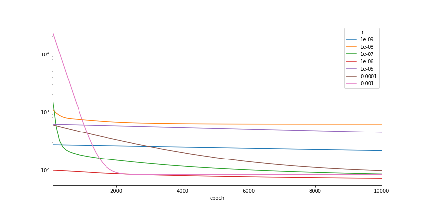
We see that with learning rate 1e-6, we can finally beat the naive baseline model, which is a constant. Wait a second, in what situation would our network be equivalent to a constant? Only if the activations are mostly zeros, and thus the model would almost always output the bias term from the last layer. Let’s see if that is the case.
model, history = train(MLP(4, 1), GradientDescent(1e-3))
print(model.layers[0](x_te))
print(model.layers[0](x_te) @ model.layers[1].variables[0])
print(model.layers[1].variables[1])
tf.Tensor(
[[0. 0. 0. 0.]
 [0. 0. 0. 0.]
 ...
 [0. 0. 0. 0.]
 [0. 0. 0. 0.]], shape=(102, 4), dtype=float32)
tf.Tensor(
[[0.]
 [0.]
 ...
 [0.]
 [0.]], shape=(102, 1), dtype=float32)
<tf.Variable 'dense_15/bias:0' shape=(1,) dtype=float32, numpy=array([22.394573], dtype=float32)>
Indeed, with learning rate 1e-3 our network basically collapsed to a bias term. In this case, the initial gradients exploded, if the learning rate is also very big, it can kill almost all the units immediately. So, we would need to either reduce the learning rate or apply some kind of control of the gradient values. Normalize the gradient is a good addition we should add to the gradient descent optimizer.
class GradientDescent(object):
    def __init__(self, lr=.01, clipnorm=None):
        self._lr = tf.Variable(lr, dtype=tf.float32)
        self.clipnorm = clipnorm

    def apply_gradients(self, grads_and_vars):
        for grad, var in grads_and_vars:
            if self.clipnorm: grad = tf.clip_by_norm(grad, self.clipnorm)
            update = - self._lr * grad
            var.assign_add(update)

model, history = train(MLP(4, 1), GradientDescent(1e-3, clipnorm=2))
ax = history.plot(x='epoch', logy=True, figsize=(12, 6))
ax.get_figure().savefig('ch4_plot_2.png')
print(history['testing_loss'].min())
49.352027893066406
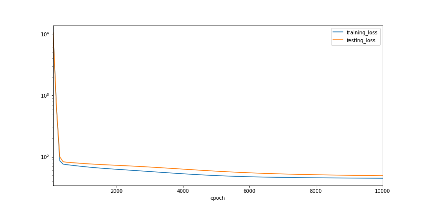
Now, we tried training our model again, this time, we normalize the gradients to have l2 norm equal to a small number 2, and indeed we got much better result even with the previously problematic learning rate value 1e-3.
2. Stochastic Gradient Descent
Yet another problem with the above gradient descent optimization is that it uses the full dataset every time it needs to do a parameter update. It can be very both very slow and memory hungry. A quick fix is to use small samples of the data to get estimates of the gradients and perform much more frequent updates. This is called stochastic gradient descent(SGD).
To train our model with SGD, we don’t need to modify our optimizer class. Instead, we need to modify the training code to include sampling. To make life a bit easier, we can wrap the data tensors into iterators.
class Dataset(object):
    def __init__(self, tensors, batch_size=32, shuffle=True):
        self.tensors = tensors if isinstance(tensors, (list, tuple)) else (tensors, )
        self.batch_size = batch_size
        self.shuffle = shuffle
        self.total = tensors[0].shape[0]
        assert all(self.total == tensor.shape[0] for tensor in self.tensors), 'Tensors should have matched length'
        self.n_steps = self.total // self.batch_size
        self._indices = tf.range(self.total)

    def __iter__(self):
        self._i = 0
        if self.shuffle:
            self._indices = tf.random.shuffle(self._indices)
        return self

    def __next__(self):
        if self._i >= self.n_steps:
            raise StopIteration
        else:
            start = self._i * self.batch_size
            end = start + self.batch_size
            indices = self._indices[start: end]
            samples = (tf.gather(tensor, indices) for tensor in self.tensors)
            self._i += 1
            return samples
With this Dataset class, we can make very small change to the training code.
train_dataset = Dataset((x_tr, y_tr))
test_dataset = Dataset((x_te, y_te))
def train(model, optimizer, n_epochs, batch_size=32, his_freq=10):
history = []
for epoch in range(1, n_epochs + 1):
tr_loss = []
for x, y in train_dataset:
tr_loss.append(train_step(model, optimizer, x, y).numpy())
te_loss = []
for x, y in test_dataset:
te_loss.append(test_step(model, x, y).numpy())
te_loss_full = test_step(model, x_te, y_te)
if not epoch % his_freq:
history.append({'epoch': epoch,
'training_loss': np.mean(tr_loss),
'testing_loss': np.mean(te_loss),
'testing_loss_full': te_loss_full.numpy()})
return model, pd.DataFrame(history)
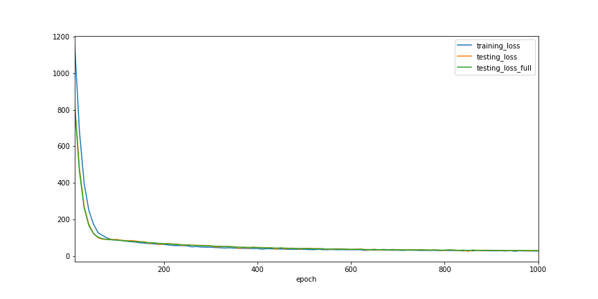
model, history = train(MLP(4, 1), GradientDescent(1e-3, 2), n_epochs=2000)
ax = history.plot(x='epoch', kind='line', figsize=(12, 6))
ax.get_figure().savefig('ch4_plot_3.png')
print(history.testing_loss_full.min())
30.624069213867188
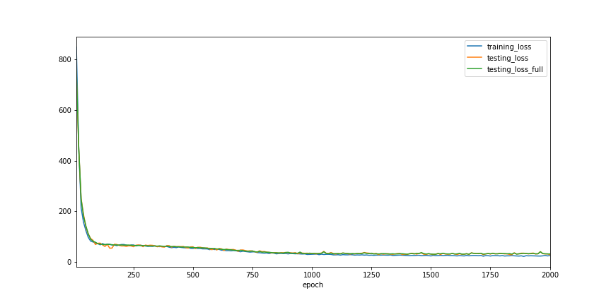
We can see that training with small batches of random samples, the trajectory of loss values becomes a bit zig-zag in shape, but still follows the similar path as previously when we train with full dataset.
3. Momentum
If we look at the learning curve, we see that after the initial huge drop, the progress becomes very slow but steady. Wondering if there is something can help us accelerate the progress? One improvement made to Gradient Descent is to accelerate it by builds up the velocity, which equals to use an exponential moving average(EMA) version of the gradients. In formula it looks like:
It is not too difficult to upgrade our gradient descent optimizer to add this feature.
class Momentum(object):
    def __init__(self, lr=.01, beta=.9, clipnorm=None):
        self._lr = tf.Variable(lr, dtype=tf.float32)
        self._beta = tf.Variable(beta, dtype=tf.float32)
        self.clipnorm = clipnorm

    def init_moments(self, var_list):
        self._moments = {var._unique_id: tf.Variable(tf.zeros_like(var))
                         for var in var_list}

    def apply_gradients(self, grads_and_vars):
        for grad, var in grads_and_vars:
            if self.clipnorm: grad = tf.clip_by_norm(grad, self.clipnorm)
            m = self._moments[var._unique_id]
            m.assign(self._beta * m - self._lr * grad)
            update = m
            var.assign_add(m)
What added a set of moment variables to accumulates gradients, and we used a mapping to keep track of the association between variables and the accumulators.
model = MLP(4, 1)
model.build(input_shape=(32,13))
optimizer = Momentum(lr=1e-3, beta=.98, clipnorm=2)
optimizer.init_moments(model.variables)
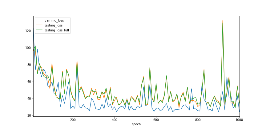
model, history = train(model, optimizer, n_epochs=1000)
ax = history.plot(x='epoch', kind='line', figsize=(12, 6))
ax.get_figure().savefig('ch4_plot_4.png')
print(history.testing_loss_full.min())
29.115631103515625
4. Second Moment
As with the first moment of the gradients, second moment were also made use to guide optimization.
The Adam optimizer looks like this in formula
In a nutshell, the optimizer uses two sets of accumulators to keep track of the first two moments of the gradients. The algorithm uses the second moment to scale the first moment, intuitively this works like a signal to noise ratio adjustment, with the first moment be the signal and the second moment be noise. Since all the operations are elementwise, this signal to noise treatment is customized for each and every parameter in the model, so effectively every parameter has its own learning rate.
With a few copy, paste and edit, we can upgrade the gradient descent with momentum optimizer to Adam easily.
class Adam(object):
    def __init__(self, lr=.01, beta_1=.9, beta_2=.999, epsilon=1e-8, clipnorm=None):
        self._lr = tf.Variable(lr, dtype=tf.float32)
        self._beta_1 = tf.Variable(beta_1, dtype=tf.float32)
        self._beta_2 = tf.Variable(beta_2, dtype=tf.float32)
        self._epsilon = tf.constant(epsilon, dtype=tf.float32)
        self.clipnorm = clipnorm
        self._t = tf.Variable(0, dtype=tf.float32)

    def init_moments(self, var_list):
        self._m = {var._unique_id: tf.Variable(tf.zeros_like(var))
                   for var in var_list}
        self._v = {var._unique_id: tf.Variable(tf.zeros_like(var))
                   for var in var_list}

    def apply_gradients(self, grads_and_vars):
        self._t.assign_add(tf.constant(1., self._t.dtype))
        for grad, var in grads_and_vars:
            if self.clipnorm: grad = tf.clip_by_norm(grad, self.clipnorm)

            m = self._m[var._unique_id]
            v = self._v[var._unique_id]

            m.assign(self._beta_1 * m + (1. - self._beta_1) * grad)
            v.assign(self._beta_2 * v + (1. - self._beta_2) * tf.square(grad))

            lr = self._lr * tf.sqrt(1 - tf.pow(self._beta_2, self._t)) / (1 - tf.pow(self._beta_1, self._t))
            update = -lr * m / (tf.sqrt(v) + self._epsilon)
            var.assign_add(update)
Let’s see if we can get better result with Adam.
model = MLP(4, 1)
model.build(input_shape=(32,13))
optimizer = Adam(lr=1e-3, beta_1=.9, beta_2=.999, epsilon=1e-8, clipnorm=2)
optimizer.init_moments(model.variables)

model, history = train(model, optimizer, n_epochs=1000)
ax = history.plot(x='epoch', kind='line', figsize=(12, 6))
ax.get_figure().savefig('ch4_plot_5.png')

print(history.testing_loss_full.min())
28.03963851928711
Adam is pretty much the default first choice of optimizer for most people on most problems. Since we have already organically coded it up, we can now take a look at how we can go about to do it by sub classing the tf.keras.optimizers.Optimizer.
To implement a custom tf.keras optimizer, there are a few methods we need to implement:
_resource_apply_dense()- this is the method used to perform parameter updates with dense gradient tensors._resource_apply_sparse()- above but works with sparse gradient tensors._create_slots()- optionally if the optimizer require more variables. If the optimizer only uses gradients and variables(like SGD), this is not needed.- ` _get_config()` - optionally for save(serialize) / load(de-serialize) the optimizer with hyperparameters.
our init_moments() method roughly corresponds to the _create_slots() and our apply_gradients() method needs to be moved to _resource_apply_dense(). And since we have quite a few hyperparameters, we need to code up the _get_config() method too.
class Adam(tf.keras.optimizers.Optimizer):
    def __init__(self, learning_rate=.001, beta_1=.9, beta_2=.999, epsilon=1e-8, name='Adam', **kwargs):
        super().__init__(name, **kwargs)
        self._set_hyper('learning_rate', kwargs.get('lr', learning_rate))
        self._set_hyper('beta_1', beta_1)
        self._set_hyper('beta_2', beta_2)
        self.epsilon = epsilon or tf.keras.backend.epsilon()

    def _create_slots(self, var_list):
        for var in var_list:
            self.add_slot(var, 'm')
        for var in var_list:
            self.add_slot(var, 'v')

    def _resource_apply_dense(self, grad, var):
        dtype = var.dtype.base_dtype
        t = tf.cast(self.iterations + 1, dtype)
        lr = self._decayed_lr(dtype)
        beta_1 = self._get_hyper('beta_1', dtype)
        beta_2 = self._get_hyper('beta_2', dtype)
        epsilon = tf.convert_to_tensor(self.epsilon, dtype)

        m = self.get_slot(var, 'm')
        v = self.get_slot(var, 'v')

        m = m.assign(beta_1 * m + (1. - beta_1) * grad)
        v = v.assign(beta_2 * v + (1. - beta_2) * tf.square(grad))

        lr = lr * tf.sqrt(1 - tf.pow(beta_2, t)) / (1 - tf.pow(beta_1, t))
        update = -lr * m / (tf.sqrt(v) + epsilon)
        var_update = var.assign_add(update)
        updates = [var_update, m, v]
        return tf.group(*updates)

    def get_config(self):
        config = super().get_config()
        config.update({
            'learning_rate': self._serialize_hyperparameter('learning_rate'),
            'beta_1': self._serialize_hyperparameter('beta_1'),
            'beta_2': self._serialize_hyperparameter('beta_2'),
            'epsilon': self.epsilon,
            'total_steps': self._serialize_hyperparameter('total_steps'),
        })
        return config
Time to see how does it compares.
model = MLP(4, 1)
optimizer = Adam(lr=1e-3, beta_1=.9, beta_2=.999, epsilon=1e-8)

model, history = train(model, optimizer, n_epochs=1000)
ax = history.plot(x='epoch', kind='line', figsize=(12, 6))
ax.get_figure().savefig('ch4_plot_5.png')

print(history.testing_loss_full.min())
29.335590362548828
From now on, we will just use tf.keras.optimizers.Adam whenever we are going to train a model.
So we spent a lot time in optimizers in this chapter, along the way we looked at the effect of learning rate, normalization of the gradient values to prevent network collapse, and looked into the black box of how a few classic optimizer works. And we see all these has a positive impact on the training result, as our network is fitted much better compare to at the end of last chapter. Next we will look into Loss functions.